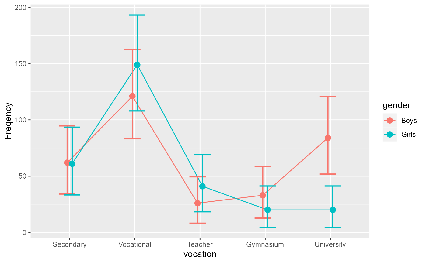
The data, taken from Light and Margolin (1971) , is an example where the educational aspiration of a large sample of N = 617 adolescents. The participants are classified by their gender (2 levels) and by their educational aspiration ( complete secondary school, complete vocational training, become college teacher, complete gymnasium, or complete university; 5 levels).
LightMargolin1971Format
An object of class data.frame.
References
Light RJ, Margolin BH (1971). “An Analysis of Variance for Categorical Data.” Journal of the American Statistical Association, 66, 534–544. doi:10.1080/01621459.1971.10482297 .
Examples
library(ANOFA)

options(superb.feedback = 'none') # shut down 'warnings' and 'design' interpretation messages

# Lets run the analysis
L <- anofa( obsfreq ~ vocation * gender, LightMargolin1971)
summary(L)
#>                       G df Gcorrected pvalue    etasq
#> Total           266.889  9         NA     NA       NA
#> vocation        215.016  4    214.668 0.0000 0.258428
#> gender            1.986  1      1.985 0.1589 0.003209
#> vocation:gender  49.887  4     49.555 0.0000 0.301949

# a quick plot
anofaPlot(L)


# Some simple effects.
e <- emFrequencies(L, ~ gender | vocation )
summary(e)
#>                            G df Gcorrected pvalue    etasq
#> gender | Secondary   0.00813  1   0.008124 1.0000 0.000066
#> gender | Vocational  2.90893  1   2.906575 0.5736 0.010659
#> gender | Teacher     3.38684  1   3.384098 0.4957 0.048118
#> gender | Gymnasium   3.22145  1   3.218840 0.5219 0.057299
#> gender | University 42.34782  1  42.313530 0.0000 0.289364

# some contrasts:
e <- emFrequencies(L, ~ vocation | gender )
f <- contrastFrequencies(e, list(
            "teacher college vs. gymnasium"=c( 0, 0, 1,-1, 0),
            "vocational vs. university"   = c( 0, 1, 0, 0,-1),
            "another"                     = c( 0, 1,-1,-1,+1)/2,
            "to exhaust the df"           = c( 4,-1,-1,-1,-1)/4
            )
        )