Unequal variances, Welch test, Tryon adjustment,
and superb
Source: vignettes/Vignette7.Rmd
Vignette7.RmdWhen the group’s variances are heterogeneous, it may results in error bars of differing length. It is then possible than one of the error bar includes the other mean, but that the second error bar does not. What can we conclude in such circumstances? This vignette explores this questions, examining Welch test solution, and Tryon adjustment along the way.
A simple example
Consider this example where two groups have been examined. Herein, the sample sizes are equal, but what follows does not depends on this.
grp1 <- c( 56,  54,  73,  46,  59,  62,  55,  53,  77,  60,  69,  66,  63,
           62,  53,  82,  74,  70,  65,  70,  72,  65,  56,  58,  83)
grp2 <- c( 51,  99, 194, 123,  40,  83,  87, 117,  46,  89,  61,  81,  53,
          141,  52,  53,  39,  96,  14,  81,  63,  66,  80, 113,  82)
These two groups have means of 64.12 and 80.16. However, they also have quite differing standard deviations, 9.493 and 37.918. The second is over four times larger than the first, which denotes a very heterogeneous variance situation.
Let’s reunite the scores of these two datasets in a
single data frame with a group indicator so that we can do
a first plot:
dtaHetero <- data.frame( cbind(
    id    = 1:(length(grp1)+length(grp2)),
    group = c(rep(1,length(grp1)), rep(2, length(grp2)) ),
    score = c(grp1, grp2)
))
head(dtaHetero)
## id group score
## 1 1 1 56
## 2 2 1 54
## 3 3 1 73
## 4 4 1 46
## 5 5 1 59
## 6 6 1 62(just to make the plots look nicer, I prepare some directives that will be added to these:
library(superb)             # to make the summary plot
library(ggplot2)            # for all the graphic directives
library(gridExtra)          # for grid.arrange

ornate = list(
    xlab("Difference"),
    scale_x_discrete(labels=c("Pre-\nTreatment","Post-\nTreatment")),
    ylab("Score"),
    coord_cartesian( ylim = c(40,+110) ),
    theme_light(base_size = 10) +
    theme( plot.subtitle = element_text(size=16))
)
). We are now ready to make a first plot. The adjustment
purpose = "difference" is necessary as we plan to compare
the two results.
pt <- superb(
            score ~ group,
            dtaHetero,
            adjustments = list(purpose = "difference"),
            gamma       = 0.95,
            statistic   = "mean",
            errorbar    = "CI",
            plotLayout  = "line",
            lineParams  = list(alpha = 0) #the line is made transparent
) + ornate
## superb::ADVICE: Some of the groups' variances are heterogeneous. Consider using purpose="tryon".
pt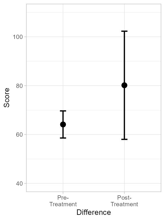
Figure 1. Plot of dtaHerero showing heterogeneous error bars.
As seen, the two error bars deliver a different message: the left one suggests a huge difference between the means, the right one does not. How do we settle this?
Averaging the error bars, sort of…
Error bars are depiction of an error variance. However, they are actually based on the standard errors which are the square root of the error variances.
Standard errors cannot be sumed (or averaged), only error variances can. Thus, when averaging the two error bars, it is their squares that must be averaged (followed by a square root). This operation is called the mean in the square sense. It is denoted mean* hereafter.
Given that the first error bar is given by and the second, by , where is the average of the group and is the standard error of the the group, averaging the error bar lengths can be simplified to
Hence, asking if the lag between the two groups is significant is actually asking
which is precisely the definition of a Welch test (Welch, 1947).
In other word, when appraising the general length of the error bars, you are actually performing a Welch test. This test is arguably the only mean test we need (Delacre, Lakens, & Leys, 2017).
A real Welch test with your eyes
Actually, the above is not entirely true, as the degrees of freedom of the multiplier is only based on the number of observations in each group ().
To really have a Welch test, it is necessary to (1) pool the degrees of freedom of the groups together; (2) rectify this degree of freedom based on the amount of heterogeneity in the data.
To get the rectified degrees of freedom according to Welch, you can issue
# Welch's rectified degrees of freedom
wdf <- WelchDegreeOfFreedom(dtaHetero, "score","group")
in which "score" is the column(s) containing the
dependent variable(s) and "group" is the column(s)
containing the group identifiers. Here, the result is 26.9965 (compared
to
,
that is 48, indicating a fairly large reduction in degree of freedom
caused by a fairly important heterogeneity.
In superb, it is possible to override the default degree
of freedom using the error bar estimator
errorbar = CIwithDF" and then in the gamma
argument, use a vector with both the confidence level desired and the
rectified degree of freedom, as in
gamma = c(0.95, 26.9965). Lets have a small plot of
this:
pw <- superb(
            score ~ group,
            dtaHetero,
            adjustments = list(purpose = "difference"),
            gamma       = c(0.95, wdf),         # new!
            statistic   = "mean",
            errorbar    = "CIwithDF",           # new!
            plotLayout  = "halfwidthline",
            lineParams  = list(alpha = 0)
) + ornate
## superb::ADVICE: Some of the groups' variances are heterogeneous. Consider using purpose="tryon".
pw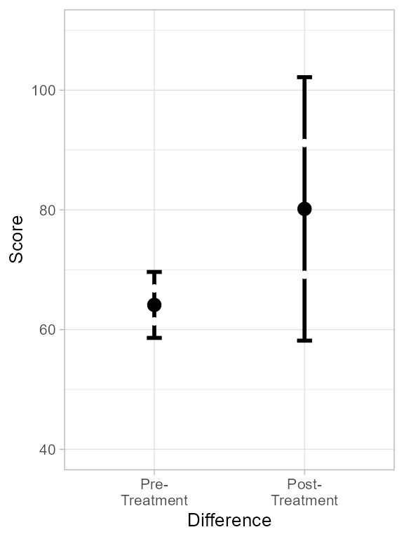
Figure 2. Plot of dtaHerero with rectified degree of freedom.
In this plot, I used a different layout, the
"halfwidthline" which shows the mid-point of the error bar
with a small gap. We will see the reason for that in a minute.
Averaging in the square sense, do you expect me to do that visually?
Averaging visually two lengths is already difficult, if it needs to be done in the square sense, that may be impossible… When averaging in the square sense, the longer lines have a stronger influence on the means so that ignoring this fact, we would tend to underestimate the mean length.
The first solution is not to bother. The usual average and the average in the square sense returns sensibly the same length. Therefore, if your results are not ambiguous, there is no need to worry any more.
The second solution is to adjust the error bar length so that they are amenable to the usual average. This is actually what Tryon’s adjustment does (Tryon, 2001). When the variances are truly homogeneous, the correction for examining pair-wise comparision is an increase by a factor of . When we deviate from homogeneity, Tryon’s adjustment tends to be a little larger than 1.41 to compensate for the underestimation introduced by regular averaging. This transformation is right on so that the usual mean of the two error bars, following a Tryon transformation, will precisely indicate whether the means are included in the mean error bar length.
pwt <- superb(
            score ~ group,
            dtaHetero,
            adjustments = list(purpose = "tryon"), #new!
            gamma       = c(0.95, wdf),
            statistic   = "mean",
            errorbar    = "CIwithDF",
            plotLayout  = "halfwidthline",
            lineParams  = list(alpha = 0)
)+ ornate
## superb::FYI: The tryon adjustments per measures are Measure 1: 1.6489 , all compared to 1.4142.
pwt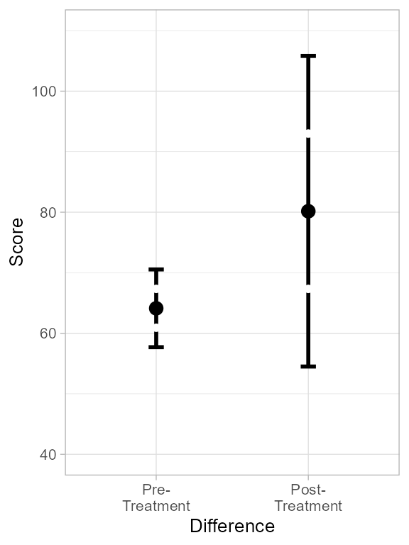
Figure 3. Plot of dtaHerero with rectified degree of freedom and Tryon’ difference-adjusted error bars.
Finally, are the groups different or not?
Let’s return to the whole question that motivated this vignette.
If we used the difference-adjusted error bars, then we need to average in the square sense the error bars. Lets do that:
# get the summary statistics with superbData
t <- superb(
            score ~ group,
            dtaHetero,
            adjustments = list(purpose = "difference"),
            gamma       = 0.95,
            statistic   = "mean", errorbar = "CI",
            showPlot    = FALSE
)
## superb::ADVICE: Some of the groups' variances are heterogeneous. Consider using purpose="tryon".
# keep only the summary statistics:
t2 <- t$summaryStatistics

# the length is in column "upperwidth", for lines 1 and 2,
# so lets do the mean in the square sense:
tmean2 <- sqrt( (t2$upperwidth[1]^2 + t2$upperwidth[2]^2)/2 )
which equals 16.135. By comparison, here is the regular mean:
tmean <- (t2$upperwidth[1] + t2$upperwidth[2] )/2which equals 13.838. This shows that in the present case, the usual average of the error bars is a length too short compared to the adequate average (in the square sense).
We’ll add a line segment of that length in the subsequent plot. Let’s do the same following Tryon’s adjusment and Welch rectified degrees of freedom:
# get the summary statistics with superbData
wt <- superb(
            score ~ group,
            dtaHetero,
            adjustments = list(purpose = "tryon"),
            gamma       = c(0.95, wdf),
            statistic   = "mean", errorbar = "CIwithDF",
            showPlot    = FALSE
)
## superb::FYI: The tryon adjustments per measures are Measure 1: 1.6489 , all compared to 1.4142.
wt2 <- wt$summaryStatistics
wmean <- (wt2$upperwidth[1]+wt2$upperwidth[2]) / 2
As seen, both length are very similar, 16.135 for the first, and 16.041 for the second. The small difference comes from the fact that in the Tryon-adjusted error bars, the degree of freedom were rectified by Welch’s formula rather than being unpooled.
With Tryon’s adjustment, the length can be averaged, which means that
half of each length totalizes the average length: this is where the
halfwidthline error bars come handy: we see the half of
their length. Hence, if they are aligned, their sum is exactly equal to
the lag between the two means.
Lets represent all this:
# showing all three plots, with reference lines in red
grid.arrange(
    pt + labs(subtitle="Difference-adjusted 95% CI\n with default degree of freedom") +
        geom_text( x = 1.15, y = mean(grp1)+(mean(grp2)-mean(grp1))/2, label = "power-2 mean", angle = 90) +
        geom_text( x = 1.55, y = mean(grp1)+(mean(grp2)-mean(grp1))/2, label = "regular mean", angle = 90) +
        geom_hline(yintercept = mean(grp1)+(mean(grp2)-mean(grp1))/2-tmean2/2, colour = "red", linewidth = 0.5, linetype=2) +
        geom_hline(yintercept = mean(grp1)+(mean(grp2)-mean(grp1))/2+tmean2/2, colour = "red", linewidth = 0.5, linetype=2) +
        # arrow for the power-2 mean
        geom_segment(arrow = arrow(length =unit(0.4,"cm")), x=1.33, y=mean(grp1)+(mean(grp2)-mean(grp1))/2,
                xend=1.33, yend=mean(grp1)+(mean(grp2)-mean(grp1))/2+tmean2/2) +
        geom_segment(arrow = arrow(length =unit(0.4,"cm")), x=1.333, y=mean(grp1)+(mean(grp2)-mean(grp1))/2,
                xend=1.33, yend=mean(grp1)+(mean(grp2)-mean(grp1))/2-tmean2/2) +
        # arrow for the regular mean
        geom_segment(arrow = arrow(length =unit(0.4,"cm")), x=1.66, y=mean(grp1)+(mean(grp2)-mean(grp1))/2,
                xend=1.66, yend=mean(grp1)+(mean(grp2)-mean(grp1))/2+tmean/2) +
        geom_segment(arrow = arrow(length =unit(0.4,"cm")), x=1.66, y=mean(grp1)+(mean(grp2)-mean(grp1))/2,
                xend=1.66, yend=mean(grp1)+(mean(grp2)-mean(grp1))/2-tmean/2),
    pw  + labs(subtitle="Difference-adjusted 95% CI\nwith df from Welch"),

    pwt + labs(subtitle="Tryon-adjusted 95% CI\nwith df from Welch") +
        geom_hline(yintercept = mean(grp1)+wt2$upperwidth[1]/2, colour = "red", linewidth = 0.5, linetype=2) +
        geom_hline(yintercept = mean(grp2)+wt2$lowerwidth[2]/2, colour = "red", linewidth = 0.5, linetype=2),
 ncol=3)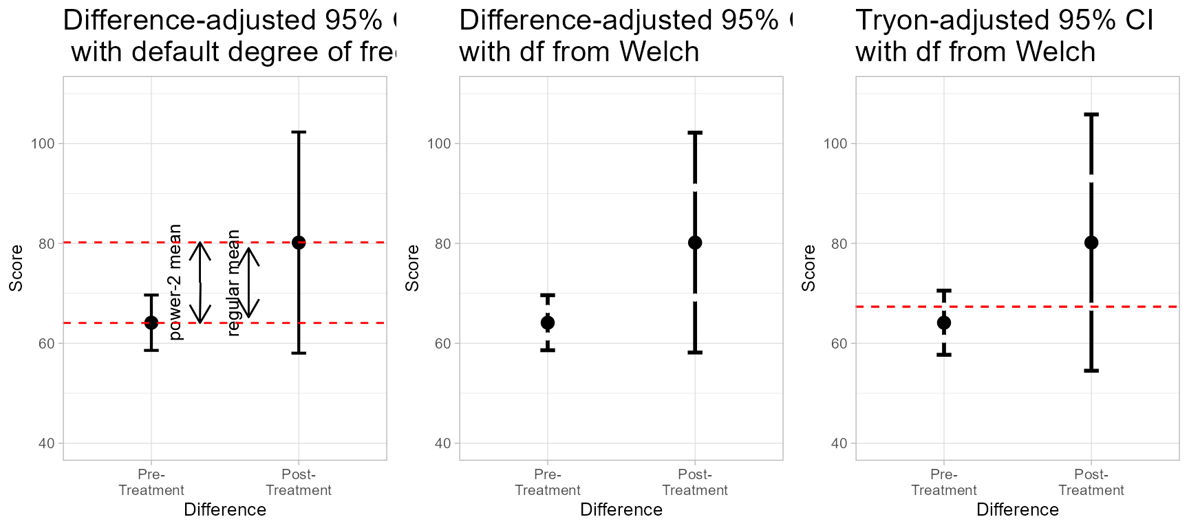
Figure 4. All three plots with relevant markers in red.
From the Tryon-adjusted confidence intervals, we see that the average length is precisely the lag between the means. In other word, the two groups are borderline significantly different. Still not convinced? Let’s do a Welch test:
t.test( grp1, grp2,
        var.equal=FALSE)
##
## Welch Two Sample t-test
##
## data: grp1 and grp2
## t = -2.0518, df = 26.996, p-value = 0.05001
## alternative hypothesis: true difference in means is not equal to 0
## 95 percent confidence interval:
## -3.208072e+01 7.239399e-04
## sample estimates:
## mean of x mean of y
## 64.12 80.16The difference is right on the limit of significance at the .05 level, mirroring the 95% confidence level used in the plot.
In summary
superb is making error bars from separate error
estimations. Hence, whenever the sample sizes are quite unequal, the
variances are quite heterogeneous, or both, the inference performed by
eyes are actually the same as performing a Welch test of means. When
both samples sizes are equal and variances are homogeneouse, there is no
difference between a Welch test and a t test.
When the degree of freedom are rectified and Tryon’s ajustment is used, the center of both confidence intervals should be exactly aligned to indicate that their mean fills exactly the gap.
Although the Tryon/Welch pair lets you make very precise inferences, visually and practically speaking, the difference between the rectified Welch degree of freedom adjustments and a plot with the default degree of freedom are undetectable (as evidence by the first plot and the second plot of Figure 4 just above).
If you can perform average in the square sense, the difference adjustment is perfect. In doubt, consider applying the Tryon adjustment when the variances are cleary heterogeneous.