![]()
The library superb offers two main functionalities. The first and foremost functionnality is to obtain plots with adjusted error bars. The main function is superb() but you can also use superbShiny() for a graphical user interface requiring no programming nor scripting. See the nice tutorial by Walker (2021).
The purpose of the function superb() is to provide a plot with summary statistics and correct error bars. With simple adjustments, the error bar are adjusted to the design (within or between), to the purpose (single, i.e., in isolation, or difference, i.e., for pair-wise comparisons), to the sampling method (simple randomized samples or cluster randomized samples) and to the population size (infinite or of a specific size). The superb(..., showPlot=FALSE) argument does not generate the plot but returns the summary statistics and the interval boundaries. These can afterwards be sent to other plotting environments.
The second, subsidiary, functionality is to Generate Random Datasets. The function GRD() is used to easily generate random data from any design (within or between) using any population distribution with any parameters, and with various effect sizes. GRD() is quite handy to test statistical procedures and plotting procedures such as superb().
Installation
The official CRAN version can be installed with
install.packages("superb")
library(superb)
The development version 1.0.1 can be accessed through GitHub:
devtools::install_github("dcousin3/superb")
library(superb)
Examples
The easiest is to use the graphical interface which can be launched with
The following examples use the script-based commands.
Here is a simple example illustrating the ToothGrowth dataset of rats (in which the dependent variable is len) as a function of the dose of vitamin and the form of the vitamin supplements supp (pills or juice)
superb(len ~ dose + supp, ToothGrowth )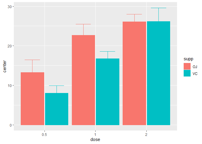
Figure 1. A simple superb plot
In the above, the default summary statistic, the mean, is used. The error bars are, by default, the 95% confidence intervals (of the mean). These two choices can be changed with the statistic and the errorbar arguments.
This second example explicitly indicates to display the median instead of the default mean summary statistics along with the default 95% confidence interval of the median here (the correct function is automatically selected):
superb(len ~ dose + supp, ToothGrowth,
    statistic = "median")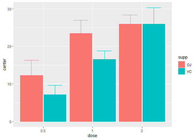
Figure 2. A median superb plot
As a third example, we illustrate the harmonic means hmean along with 99.9% confidence intervals of the harmonic mean displayed using bars:
superb(len ~ dose + supp, ToothGrowth,
    statistic = "hmean",
    errorbar = "CI", gamma = 0.999,
    plotLayout = "bar")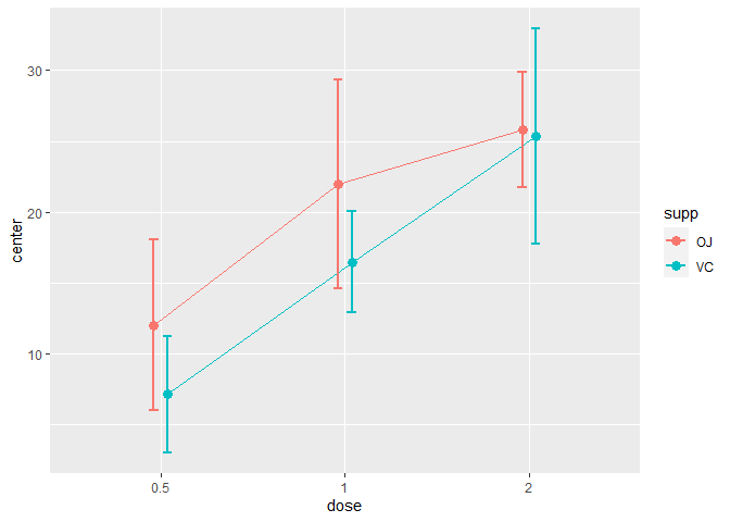
Figure 4. A simple superb plot with 99.9%CI
The second function, GRD(), can be used to generate random data from designs with various within- and between-subject factors. This example generates scores for 30 simulated participants in a 3 x 6 design with 6 daily repeated-measures on Days. The factor Day is modeled as impacting the scores (increasing by 3 points per day) whereas difficulty is beneficial for the C level only:
set.seed(663) # for reproducibility
testdata <- GRD(
    RenameDV   = "score",
    SubjectsPerGroup = 10,
    BSFactors  = "Difficulty(A,B,C)",
    WSFactors  = "Day(6)",
    Population = list(mean = 75,stddev = 10,rho = 0.8),
    Effects    = list( "Difficulty" =  custom(-5,-5,+10), "Day" = slope(3) )
)
head(testdata)
## id Difficulty score.1 score.2 score.3 score.4 score.5 score.6
## 1 1 A 61.72393 61.48460 70.48406 68.92430 69.85908 68.15339
## 2 2 A 54.16784 65.82688 66.51785 65.59598 82.74906 82.53300
## 3 3 A 69.85369 60.04088 73.99657 72.95358 69.89209 74.30423
## 4 4 A 69.05319 64.99568 75.00310 78.35253 81.48167 76.08335
## 5 5 A 79.29388 81.56254 78.17444 86.36108 92.45310 93.73091
## 6 6 A 56.56657 59.23395 66.10074 63.77299 67.07331 72.64133This is here that the full benefits of superb() is seen: with just a few adjustments, you can obtained decorrelated error bars with the Correlation-adjusted (CA), the Cousineau-Morey (CM) or the Loftus & Masson (CM) techniques:
library(gridExtra)          # for grid.arrange
library(RColorBrewer)       # for nicer color palette

plt1 <- superb( crange(score.1, score.6) ~ Difficulty,
    testdata, WSFactors = "Day(6)",
    plotLayout = "line"
) + ylim(50,100) + labs(title = "No adjustments") +
theme_bw() + ylab("Score") +
scale_color_brewer(palette="Dark2")

plt2 <- superb( crange(score.1, score.6) ~ Difficulty,
    testdata, WSFactors = "Day(6)",
    adjustments = list(purpose = "difference", decorrelation = "CA"),
    plotLayout = "line"
)+ ylim(50,100) + labs(title = "correlation- and difference-adjusted") +
theme_bw() + ylab("Score") +
scale_color_brewer(palette="Dark2")

grid.arrange(plt1,plt2, ncol=2)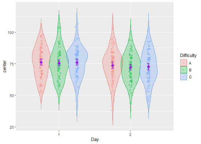
Figure 4. Multiple superb plots
Even better, the simulated scores can be illustrated using more elaborate layouts such as the pointjitter layout which, in addition to the mean and confidence interval, shows the raw data using jitter dots:
superb( crange(score.1, score.6) ~ Difficulty,
    testdata, WSFactors = "Day(6)",
    adjustments = list(purpose = "difference", decorrelation = "CM"),
    plotLayout = "pointjitter",
    errorbarParams = list(color = "purple"),
    pointParams = list( size = 3, color = "purple")
) +
theme_bw() + ylab("Score") +
scale_color_brewer(palette="Dark2")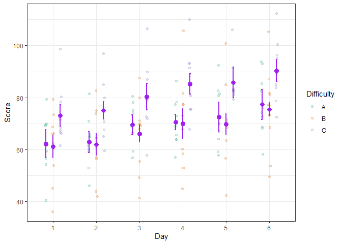
Figure 5. A decorated superb plot
In the above example, optional arguments errorbarParams and pointParams are used to inject specifications in the error bars and the points respectively. When these arguments are used, they override the defaults from superb().
Lastly, we could aim for a radar (a.k.a. circular) plot with
superb( crange(score.1, score.6) ~ Difficulty, testdata,
    WSFactors = "Day(6)",
    adjustments = list(purpose = "difference", decorrelation = "CM"),
    plotLayout = "circularpointlinejitter",
    factorOrder = c("Day", "Difficulty"),
    pointParams = list( size = 3 ),
    jitterParams = list(alpha=0.25),
    errorbarParams= list(width=0.33, color = "black")
) +
theme_bw() + ylab("") +
theme(panel.border = element_blank(), text = element_text(size = 16) ) +
scale_color_brewer(palette="Dark2") +
theme(axis.line.y = element_blank(),
axis.text.y=element_blank(), axis.ticks.y=element_blank())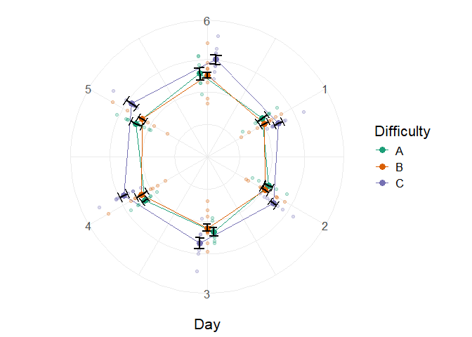
Figure 6. A simple superb plot
Every time, you get error bars for free! no need to compute them on the side, no need to worry about the adjustments (whether you want stand-alone error bars or adjusted for purpose or correlation, it is all just one option). Also, keep in mind that it is easy to change the default (mean +- 95% confidence intervals) to any other summary statistics –e.g., median– and any other measure of error –e.g., standard error, standard deviation, inter-quartile range, name it–; you can find some responses in the vignettes or on stackExchange or just open an issue on the github repository.
For more
superb is for summary plot with error bars, as simple as that.
The library superb makes it easy to illustrate summary statistics along with error bars. Some layouts can be used to visualize additional characteristics of the raw data. Finally, the resulting appearance can be customized in various ways.
The complete documentation is available on this site.
A general introduction to the superb framework underlying this library is published at Advances in Methods and Practices in Psychological Sciences (Cousineau, Goulet, & Harding, 2021). Also, most of the formulas for confidence intervals when statistics other than the mean are displayed can be found in Harding, Tremblay, & Cousineau (2015).