(advanced) Non-factorial within-subject designs in superb

In this vignette, we show how to display a dataset with a non-full factorial within-subject design. A non-factorial design is when all the levels of a first factor are not fully crossed with all the levels of a second factor. For example, if you have a design \(A(4) \times B(4)\), you would expect in total 16 levels in a full-factorial design. If there are fewer than 16 levels, it would mean that some combinations were not measured. This could be because these conditions are uninteresting or impossible.

In a between group design, non full-factorial designs are not problematic: the columns contains the level of the factors. If some levels are missing, it just results in a shorter data file. All the levels present are fully identifiable as the levels are in these columns.

In within-subject design, this is a different matter: the columns must be matched to a condition. If some columns are missing, superb cannot guess which levels are present and which are absent. It is therefore necessary to specify what levels the columns represent.

An example

Consider a case where participants are presented with strings of 1 to 4 letters for which a decision must be made, e.g., Is this a real word?. The strings can be composed of a variable number of letters between 1 and 4, but also, with a variable number of upper-case letters, between 1 and 4. All the combinations of string length and uppercase are presented within subjects.

This design cannot be a a full factorial design. Indeed, when 1 letter is presented, it is not possible that the number of upper-case letter be 2, 3 or 4.

To handle that case, it is possible to specify a WSDesign argument. By default, this argument is "fullfactorial". When not full factorial, a list is given with, for each variables used as dependent variable, the levels of the factors they correspond.

Consider this table with number of letters presented (from 1 to 4), and number of upper-case letters (from 1 to all). The valid cases are

	Nletters	Nuppercase
var1	1	1
var2	2	1
var3	3	1
var4	4	1
var5	2	2
var6	3	2
var7	4	2
var8	3	3
var9	4	3
var10	4	4

There are 10 conditions (instead of the \(4 \times 4\) if the design had been full factorial). The table provide for each variables the levels of the two factors they correspond to.

Informing superb of a non-full factorial within-subject design

In superb(), superbPlot() or superbData(), we indicate non full factorial design with:

WSFactors = c("Nletters","Nuppercase"),
variables = c("var1","var2","var3","var4","var5","var6",
                "var7","var8","var9","var10"),
WSDesign  = list(c(1,1), c(2,1), c(3,1), c(4,1), c(2,2), c(3,2),
                 c(4,2), c(3,3), c(4,3), c(4,4)),

Returning to the example

let’s try this with a random data set. It will simulate response times for participants to response Word or **Non-word* to the presented strings. As GRD() can only generate full factorial design, we will delete some columns aftewards.

Fulldta <- dta <- GRD( 
                WSFactors = c("Nletters(4)","Nuppercase(4)"),
                Effects = list("Nletters" = slope(25),
                               "Nuppercase" = slope(-25) ),
                Population = list(mean = 400, stddev = 50)
)

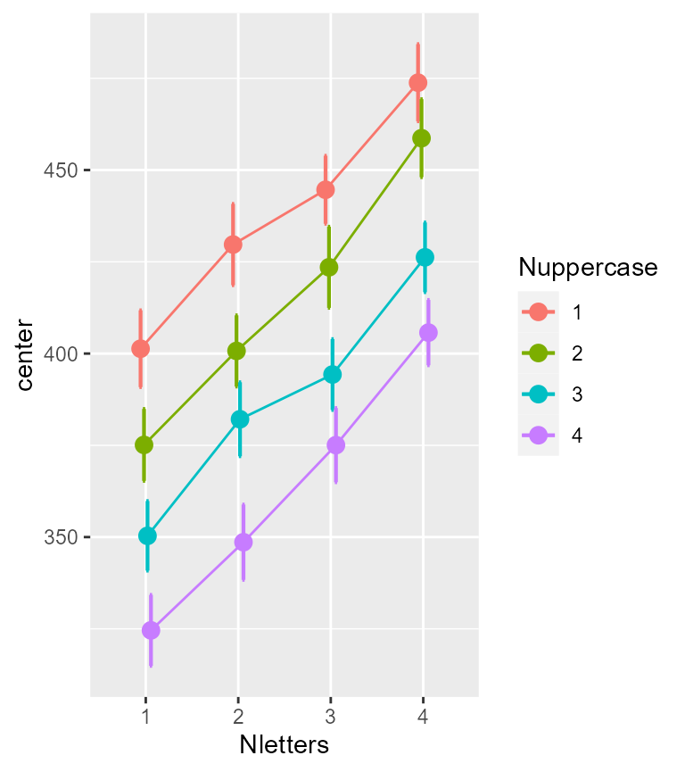
This dataset simulate an effect of the number of letters (increasing response times by 25 ms for each additional letter) and of the number of uppercase letters (decreasing response times by 25 ms for each additional uppercase letter).

The full data can be plotted without any difficulty with superbPlot():

superb(
    crange(DV.1.1, DV.4.4) ~ .,
    Fulldta,
    WSFactors = c("Nletters(4)","Nuppercase(4)"),
    plotStyle="line"
)

Figure 1. Mean response times to say Word or Non-word.

To simulate a more realistic dataset, we must remove the impossible conditions:

# destroying the six impossible columns
dta$DV.1.2 = NULL # e.g., the condition showing one letter with 2 upper-cases.
dta$DV.1.3 = NULL
dta$DV.1.4 = NULL
dta$DV.2.3 = NULL
dta$DV.2.4 = NULL
dta$DV.3.4 = NULL

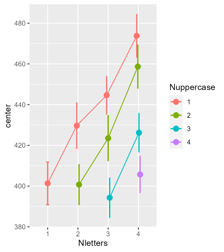
after which the plot can be performed:

superb(
    crange(DV.1.1, DV.4.4) ~ .,
    dta,
    WSFactors = c("Nletters(4)","Nuppercase(4)"),
    WSDesign  = list(c(1,1), c(2,1), c(3,1),  c(4,1),  c(2,2),  c(3,2),
                     c(4,2), c(3,3), c(4,3),  c(4,4)),
    plotStyle="line"
)

Figure 2. Mean response times to say Word or Non-word.

Really, the only new manipulation is the use of WSDesign where for each within-subject variable in the dataset, the levels of the corresponding factors (in the order they were given in WSFactors) are listed.

Note that the WSDesign levels superseeds the total number of levels, 4, given in the WSFactors. Hence, Nletters could be given as Nletters(99) or as Nletters(1), that has no longer any impact on the plot.

Also note that if the data are given in a long format, you can omit WSDesign. The long format contains enough information for superb() to correctly guess the conditions.

In summary

Full-factorial design are generally prefered as powerfull analyses can manipulate such data (for example, the ANOVA). Further, causality in experimental designs are more aptly assessed with the full-factorial design. However, it is not always possible or usefull to run a full-factorial design.