The package superb includes the function
GRD(). This function is used to easily generate random data
sets. With a few options, it is possible to obtain data from any design,
with any effects. This function, first created for SPSS Harding & Cousineau (2015) was exported to R
(Calderini & Harding, 2019). A brief
report shows one possible use in the class for teaching statistics to
undergrads (Cousineau, 2020).
This vignette illustrate some of its use.
Simplest specification
The simplest use relies on the default value:
dta <- GRD()## ------------------------------------------------------------
## Design is: with 1 independent groups.
## ------------------------------------------------------------
## 1.Between-Subject Factors ( 1 groups ) :
## 2.Within-Subject Factors ( 1 repeated measures ):
## 3.Subjects per group ( 100 total subjects ):
## 100
## ------------------------------------------------------------
head(dta)## id DV
## 1 1 -1.40004352
## 2 2 0.25531705
## 3 3 -2.43726362
## 4 4 -0.00557129
## 5 5 0.62155272
## 6 6 1.14841160By default, one hundred scores are generated from a normal
distribution with mean 0 and standard deviation of 1. In other words, it
generate 100 z scores. The dependent variable, the last column in the
dataframe that will be generated is called by default DV.
The first column is an “id” column containing a number identifying each
simulated participant. To change the dependent variable’s name,
use
dta <- GRD( RenameDV = "score" )## ------------------------------------------------------------
## Design is: with 1 independent groups.
## ------------------------------------------------------------
## 1.Between-Subject Factors ( 1 groups ) :
## 2.Within-Subject Factors ( 1 repeated measures ):
## 3.Subjects per group ( 100 total subjects ):
## 100
## ------------------------------------------------------------Data from a design with between-subject factors and within-subject factors.
To add various groups to the dataset, use the argument
BSFactors, as in
dta <- GRD( BSFactors = 'Group(3)')## ------------------------------------------------------------
## Design is: 3 with 3 independent groups.
## ------------------------------------------------------------
## 1.Between-Subject Factors ( 3 groups ) :
## Group; levels: 1, 2, 3
## 2.Within-Subject Factors ( 1 repeated measures ):
## 3.Subjects per group ( 300 total subjects ):
## 100
## ------------------------------------------------------------There will be 100 random z scores in each of three groups, for a
total of 300 data. The group number will be given in an additional
column, here called Group. A factorial design can be
generated with more than one factors, such as
## ------------------------------------------------------------
## Design is: 2 x 3 with 6 independent groups.
## ------------------------------------------------------------
## 1.Between-Subject Factors ( 6 groups ) :
## Surgery; levels: 1, 2
## Therapy; levels: 1, 2, 3
## 2.Within-Subject Factors ( 1 repeated measures ):
## 3.Subjects per group ( 600 total subjects ):
## 100
## ------------------------------------------------------------which will results in 2 3, that is, 6 different groups, crossing all the levels of Surgery (1 and 2) and all the levels of Therapy (1, 2 and 3). The levels can receive names rather than number, as in
## ------------------------------------------------------------
## Design is: 2 x 3 with 6 independent groups.
## ------------------------------------------------------------
## 1.Between-Subject Factors ( 6 groups ) :
## Surgery; levels: yes, no
## Therapy; levels: CBT, Control, Exercise
## 2.Within-Subject Factors ( 1 repeated measures ):
## 3.Subjects per group ( 600 total subjects ):
## 100
## ------------------------------------------------------------
unique(dta$Surgery)## [1] "yes" "no"
unique(dta$Therapy)## [1] "CBT" "Control" "Exercise"Finally, within-subject factors can also be given, as in
dta <- GRD(
BSFactors = c('Surgery(yes,no)', 'Therapy(CBT, Control,Exercise)'),
WSFactors = 'Contrast(C1,C2,C3)',
)## ------------------------------------------------------------
## Design is: 2 x 3 x ( 3 ) with 6 independent groups.
## ------------------------------------------------------------
## 1.Between-Subject Factors ( 6 groups ) :
## Surgery; levels: yes, no
## Therapy; levels: CBT, Control, Exercise
## 2.Within-Subject Factors ( 3 repeated measures ):
## Contrast; levels : C1, C2, C3
## 3.Subjects per group ( 600 total subjects ):
## 100
## ------------------------------------------------------------For within-subject designs, the repeated measures will appear in distinct columns (here “DV.C1”, “DV.C2”, and “DV.C3” ). This format is called wide format, meaning that the repeated measures are all on the same line for a given simulated participant.
Deciding the sample sizes
The default is to generate 100 participants in each between-subject
groups. This default can be changed with SubjectsPerGroup.
The most straigthforward specification is, e.g.,
SubjectsPerGroup = 25 for 25 participants in each groups.
Unequal group sizes can be specified with:
## ------------------------------------------------------------
## Design is: 3 with 3 independent groups.
## ------------------------------------------------------------
## 1.Between-Subject Factors ( 3 groups ) :
## Therapy; levels: 1, 2, 3
## 2.Within-Subject Factors ( 1 repeated measures ):
## 3.Subjects per group ( 8 total subjects ):
## 2 5 1
## ------------------------------------------------------------
dta## id Therapy DV
## 1 1 1 -0.03173968
## 2 2 1 -1.15996668
## 3 3 2 1.95394186
## 4 4 2 -1.79987173
## 5 5 2 -0.10192789
## 6 6 2 0.90432320
## 7 7 2 1.04921417
## 8 8 3 0.44082485Choosing the population distribution
To sample random data, it is necessary to specify a theoretical
population distribution. The default is to use a normal distribution
(the famous “bell-shaped” curve). That population has a grand mean
(GM,
)
given by the element mean and standard deviation
()
given by the element stddev. These can be redefined using
the argument Population with a list of the relevant
elements. In the following example, IQ are being simulated with :
## ------------------------------------------------------------
## Design is:  with 1 independent groups.
## ------------------------------------------------------------
## 1.Between-Subject Factors ( 1 groups ) :
## 2.Within-Subject Factors ( 1 repeated measures ):
## 3.Subjects per group ( 100 total subjects ):
##   100
##  ------------------------------------------------------------
hist(dta$IQ)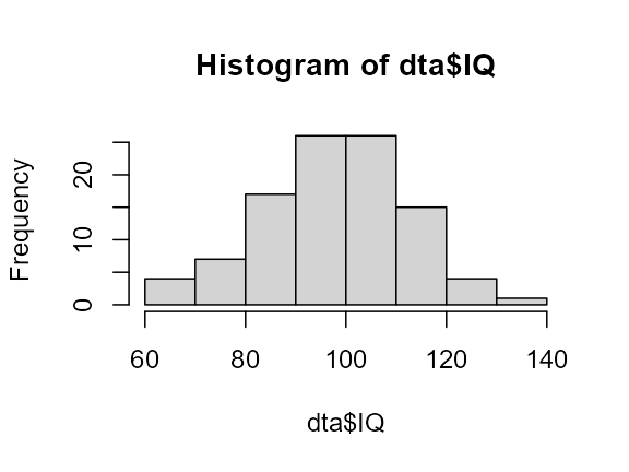
(increase the number of participants using
SubjectsPerGroup to say 10,000, and the bell-shape curve
will be evident!).
Internally, the above call to GRD() will use
rnorm to generate the scores, passing along for the mean
parameter the grand mean (internally called GM) and for the
standard deviation parameter the provided standard deviation (internally
called STDDEV). This can be explicitly stated using the
element scores as in:
dta <- GRD(
    BSFactors = "Group(2)",
    Population = list(
        mean   = 100,         # this set GM to 100
        stddev = 15,        # this set STDDEV to 15
        scores = "rnorm(1, mean = GM, sd = STDDEV )"
    )
)
## ------------------------------------------------------------
## Design is: 2 with 2 independent groups.
## ------------------------------------------------------------
## 1.Between-Subject Factors ( 2 groups ) :
## Group; levels: 1, 2
## 2.Within-Subject Factors ( 1 repeated measures ):
## 3.Subjects per group ( 200 total subjects ):
## 100
## ------------------------------------------------------------Using scores, it is possible to alter the parameters,
for example, have a mean proportional to the group number, or the
standard deviation proportional to the group number, as in:
dta <- GRD(
    BSFactors = "Group(2)",
    Population = list(
        mean   = 100,       # this set GM to 100
        stddev = 15,        # this set STDDEV to 15
        scores = "rnorm(1, mean = GM, sd = Group * STDDEV )"
    )
)
## ------------------------------------------------------------
## Design is: 2 with 2 independent groups.
## ------------------------------------------------------------
## 1.Between-Subject Factors ( 2 groups ) :
## Group; levels: 1, 2
## 2.Within-Subject Factors ( 1 repeated measures ):
## 3.Subjects per group ( 200 total subjects ):
## 100
## ------------------------------------------------------------
superb(
    DV ~ Group,
    dta,
    plotLayout = "pointjitterviolin" )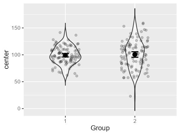
Any valid R instruction could be placed in the scores
arguments, such as
scores = "rnorm(1, mean = GM, sd = ifelse(Group==1,10,50) )"
to select the standard deviation according to Group or
scores = "1" to generate constants. Other theoretical
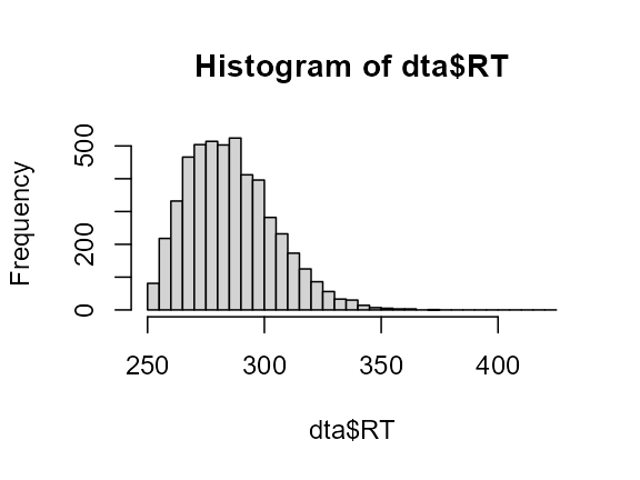
distributions can also be chosen, as in:
dta <- GRD(SubjectsPerGroup = 5000,
    RenameDV = "RT",
    Population=list(
        scores = "rweibull(1, shape=2, scale=40)+250"
    )
)
## ------------------------------------------------------------
## Design is: with 1 independent groups.
## ------------------------------------------------------------
## 1.Between-Subject Factors ( 1 groups ) :
## 2.Within-Subject Factors ( 1 repeated measures ):
## 3.Subjects per group ( 5000 total subjects ):
## 5000
## ------------------------------------------------------------
Getting effects on one or some of the factors
It is possible to generate non-null effects on the factors using the
argument Effects. Effects can be slope(x) (an
increase of x points for each level of the factor),
extent(x) (a total increase of x over all the
levels), custom(x, y, etc) for an effect of x
point for the first level of the factor, y point for the
second, etc.
Here is a slope, effect:
dta <- GRD(
    BSFactors = 'Therapy(CBT, Control, Exercise)',
    WSFactors = 'Contrast(3)',
    SubjectsPerGroup = 1000,
    Effects = list('Contrast' = slope(2))
)
## ------------------------------------------------------------
## Design is: 3 x ( 3 ) with 3 independent groups.
## ------------------------------------------------------------
## 1.Between-Subject Factors ( 3 groups ) :
## Therapy; levels: CBT, Control, Exercise
## 2.Within-Subject Factors ( 3 repeated measures ):
## Contrast; levels : 1, 2, 3
## 3.Subjects per group ( 3000 total subjects ):
## 1000
## ------------------------------------------------------------
superb(
    crange(DV.1, DV.3) ~ Therapy,
    dta,
    WSFactors = "Contrast(3)",
    plotLayout= "line" )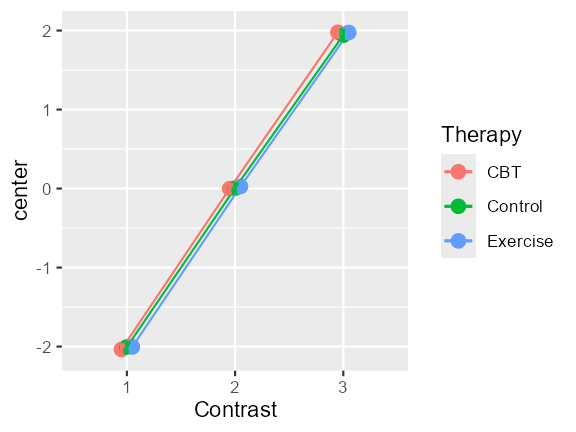
Effects can also be any R code manipulating the factors, using
Rexpression. One example:
dta <- GRD(
    BSFactors = 'Therapy(CBT,Control,Exercise)',
    WSFactors = 'Contrast(3) ',
    SubjectsPerGroup = 1000,
    Effects = list(
        "code1"=Rexpression("if (Therapy =='CBT'){-1} else {0}"),
        "code2"=Rexpression("if (Contrast ==3) {+1} else {0}")
    )
)
## ------------------------------------------------------------
## Design is: 3 x ( 3 ) with 3 independent groups.
## ------------------------------------------------------------
## 1.Between-Subject Factors ( 3 groups ) :
## Therapy; levels: CBT, Control, Exercise
## 2.Within-Subject Factors ( 3 repeated measures ):
## Contrast; levels : 1, 2, 3
## 3.Subjects per group ( 3000 total subjects ):
## 1000
## ------------------------------------------------------------
superb(
    crange(DV.1, DV.3) ~ Therapy,
    dta,
    WSFactors = "Contrast(3)",
    plotLayout= "line" )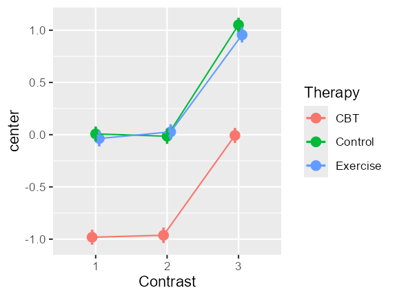
Repeated measures can also be generated from a multivariate normal
distribution with a correlation rho, with, e.g.,
dta <- GRD(
    WSFactors = 'Difficulty(1, 2)',
    SubjectsPerGroup = 1000,
    Population=list(mean = 0,stddev = 20, rho = 0.5)
)
## ------------------------------------------------------------
## Design is: ( 2 ) with 1 independent groups.
## ------------------------------------------------------------
## 1.Between-Subject Factors ( 1 groups ) :
## 2.Within-Subject Factors ( 2 repeated measures ):
## Difficulty; levels : 1, 2
## 3.Subjects per group ( 1000 total subjects ):
## 1000
## ------------------------------------------------------------
plot(dta$DV.1, dta$DV.2)
In the case of a multivariate normal distribution, the parameters for the mean and the standard deviations can be vectors of length equal to the number of repeated measures. However, covariances are constants.
dta <- GRD(
    WSFactors = 'Difficulty(1, 2)',
    SubjectsPerGroup = 1000,
    Population=list(mean = c(10,2),stddev= c(1,0.2),rho =-0.85)
)
## ------------------------------------------------------------
## Design is: ( 2 ) with 1 independent groups.
## ------------------------------------------------------------
## 1.Between-Subject Factors ( 1 groups ) :
## 2.Within-Subject Factors ( 2 repeated measures ):
## Difficulty; levels : 1, 2
## 3.Subjects per group ( 1000 total subjects ):
## 1000
## ------------------------------------------------------------
plot(dta$DV.1, dta$DV.2)
Contaminate your samples!
Contaminants can be inserted in the simulated data using
Contaminant. This argument works exactly like
Population except for the additional option
proportion which indicates the proportion of contaminants
in the samples:
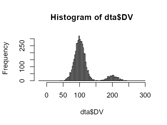
dta <- GRD(SubjectsPerGroup = 5000,
    Population= list( mean=100, stddev = 15 ),
    Contaminant=list( mean=200, stddev = 15, proportion = 0.10 )
)
## ------------------------------------------------------------
## Design is: with 1 independent groups.
## ------------------------------------------------------------
## 1.Between-Subject Factors ( 1 groups ) :
## 2.Within-Subject Factors ( 1 repeated measures ):
## 3.Subjects per group ( 5000 total subjects ):
## 5000
## ------------------------------------------------------------
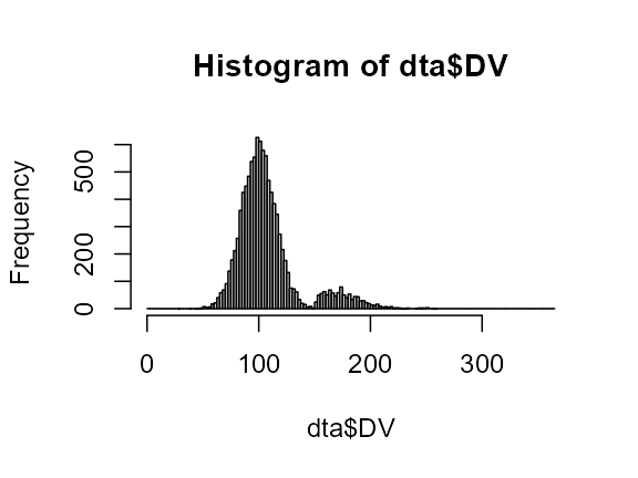
Contaminants can be normally distributed (as above) or come from any theoretical distribution which can be simulated in R:
dta <- GRD(SubjectsPerGroup = 10000,
    Population=list( mean=100, stddev = 15 ),
    Contaminant=list( proportion = 0.10,
        scores="rweibull(1,shape=1.5, scale=30)+1.5*GM")
)
## ------------------------------------------------------------
## Design is: with 1 independent groups.
## ------------------------------------------------------------
## 1.Between-Subject Factors ( 1 groups ) :
## 2.Within-Subject Factors ( 1 repeated measures ):
## 3.Subjects per group ( 10000 total subjects ):
## 10000
## ------------------------------------------------------------
Finally, contaminants can be used to add missing data (missing completely at random) with:
dta <- GRD( BSFactors="grp(2)",
    WSFactors = "Moment (2)",
    SubjectsPerGroup = 1000,
    Effects = list("grp" = slope(100) ),
    Population=list(mean=0,stddev=20,rho= -0.85),
    Contaminant=list(scores = "NA", proportion=0.2)
)
## ------------------------------------------------------------
## Design is: 2 x ( 2 ) with 2 independent groups.
## ------------------------------------------------------------
## 1.Between-Subject Factors ( 2 groups ) :
## grp; levels: 1, 2
## 2.Within-Subject Factors ( 2 repeated measures ):
## Moment; levels : 1, 2
## 3.Subjects per group ( 2000 total subjects ):
## 1000
## ------------------------------------------------------------In summary
GRD() is a convenient function to generate about any
sorts of data sets with any form of effects. The data can simulate any
factorial designs involving between-subject designs, repeated-measure
designs, and multivariate data.
One use if of course in the classroom: students can test their skill by generating random data sets and run statistical procedures. To illustrate type-I errors, it become then easy to generate data with no effect whatsoever and ask the students who obtain a rejection decision to raise their hand.