The function GRD() generates a data frame containing
random data suitable for analyses.
The data can be from within-subject or between-group designs.
Within-subject designs are in wide format. The function was originally
presented in Calderini and Harding (2019)
.
GRD(
  RenameDV = "DV",
  SubjectsPerGroup = 100,
  BSFactors = "",
  WSFactors = "",
  Effects = list(),
  Population = list(mean = 0, stddev = 1, rho = 0, scores =
    "rnorm(1, mean = GM, sd = STDDEV)"),
  Contaminant = list(mean = 0, stddev = 1, rho = 0, scores =
    "rnorm(1, mean = CGM, sd = CSTDDEV)", proportion = 0),
  Instrument = list(precision = 10^(-8), range = c(-Inf, +Inf))
)
Arguments
- RenameDV
provide a name for the dependent variable (default DV)
- SubjectsPerGroup
indicates the number of simulated scores per group (default 100 in each group)
- BSFactors
a string indicating the between-subject factor(s) with, between parenthesis, the number of levels or the list of level names. Multiple factors are separated with a colon ":" or enumerated in a vector of strings.
- WSFactors
a string indicating the within-subject factor(s) in the same format as the between-subject factors
- Effects
a list detailing the effects to apply to the data. The effects can be given with a list of
"factorname" = effect_specificationor"factorname1*factorname2" = effect_specificationpairs, in which effect_specification can either beslope(),extent(),custom()andRexpression(). For slope and extent, provide a range, for custom, indicate the deviation from the grand mean for each cell, finally, for Rexpression, give between quote any R commands which returns the deviation from the grand mean, using the factors. See the last example below.- Population
a list providing the population characteristics (default is a normal distribution with a mean of 0 and standard deviation of 1)
- Contaminant
a list providing the contaminant characteristics and the proportion of contaminant (default 0)
- Instrument
a list providing some characteristics of the measurement instrument (at this time, its precision and range only).
Value
a data.frame() with the simulated scores.
Note
Note that the range effect specification has been renamed
extent to avoid masking the base function base::range().
References
Calderini M, Harding B (2019). “GRD for R: An intuitive tool for generating random data in R.” The Quantitative Methods for Psychology, 15(1), 1–11. doi:10.20982/tqmp.15.1.p001 .
Calderini M, Harding B (2019). “GRD for R: An intuitive tool for generating random data in R.” The Quantitative Methods for Psychology, 15(1), 1–11. doi:10.20982/tqmp.15.1.p001 .
Examples
# Simplest example using all the default arguments:
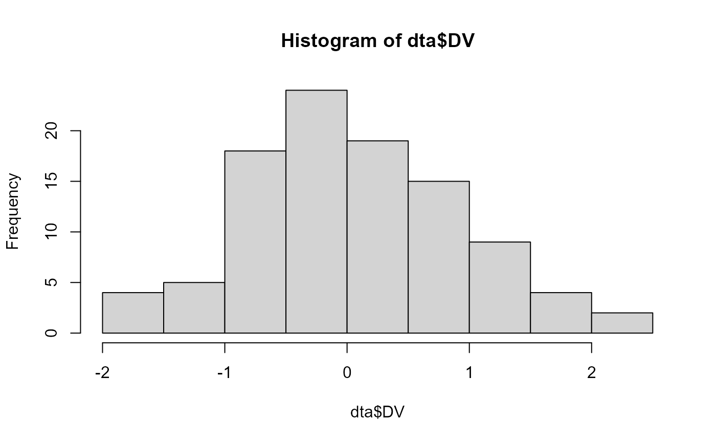
dta <- GRD()
head(dta)
#> id DV
#> 1 1 -0.0593134
#> 2 2 1.1000254
#> 3 3 0.7631757
#> 4 4 -0.1645236
#> 5 5 -0.2533617
#> 6 6 0.6969634
hist(dta$DV)
 # Renaming the dependant variable and setting the group size:
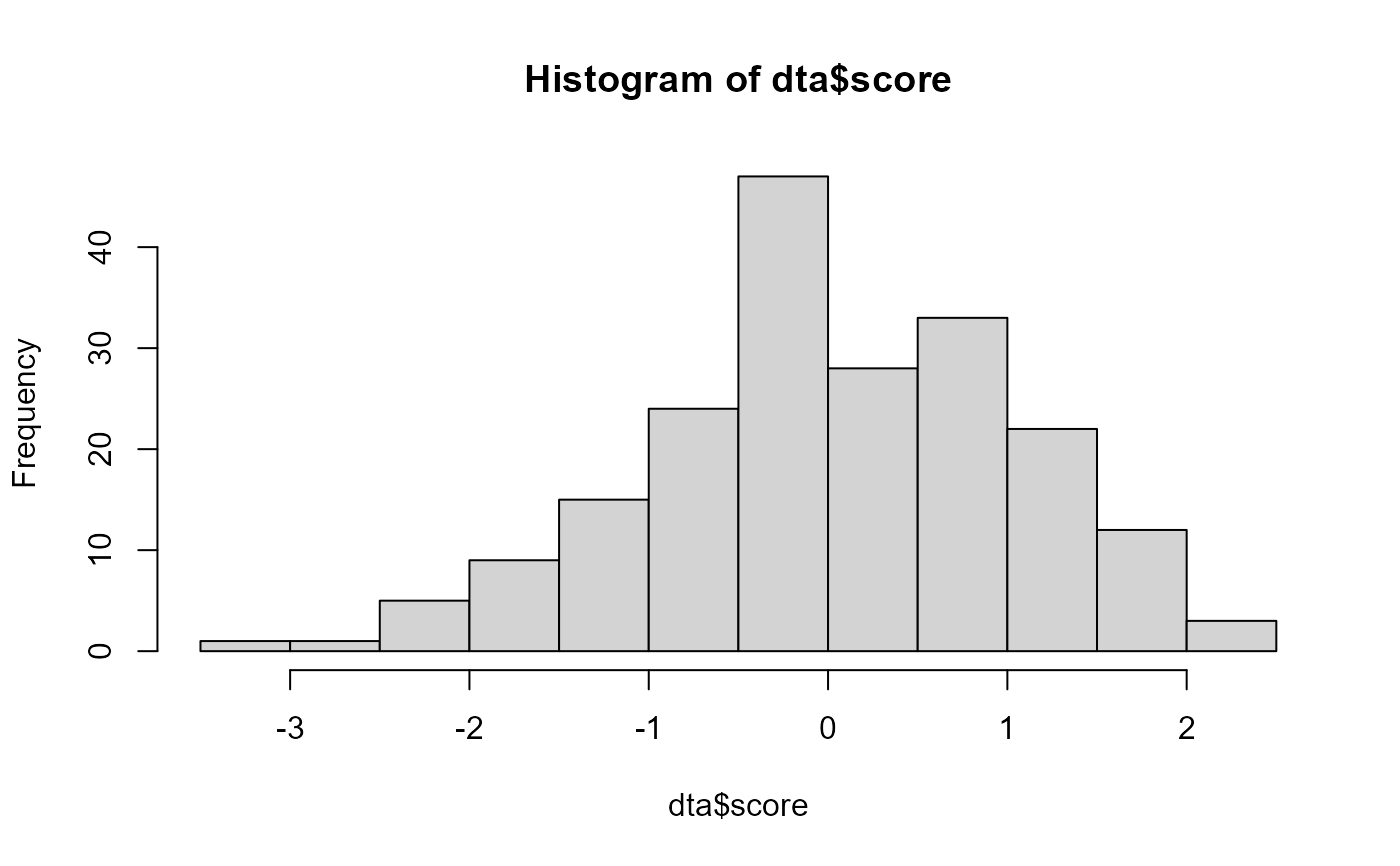
dta <- GRD( RenameDV = "score", SubjectsPerGroup = 200 )
hist(dta$score )
# Renaming the dependant variable and setting the group size:
dta <- GRD( RenameDV = "score", SubjectsPerGroup = 200 )
hist(dta$score )
 # Examples for a between-subject design and for a within-subject design:
dta <- GRD( BSFactors = '3', SubjectsPerGroup = 20)
dta <- GRD( WSFactors = "Moment (2)", SubjectsPerGroup = 20)
# A complex, 3 x 2 x (2) mixed design with a variable amount of participants in the 6 groups:
dta <- GRD(BSFactors = "difficulty(3) : gender (2)",
WSFactors="day(2)",
SubjectsPerGroup=c(20,24,12,13,28,29)
)
# Defining population characteristics :
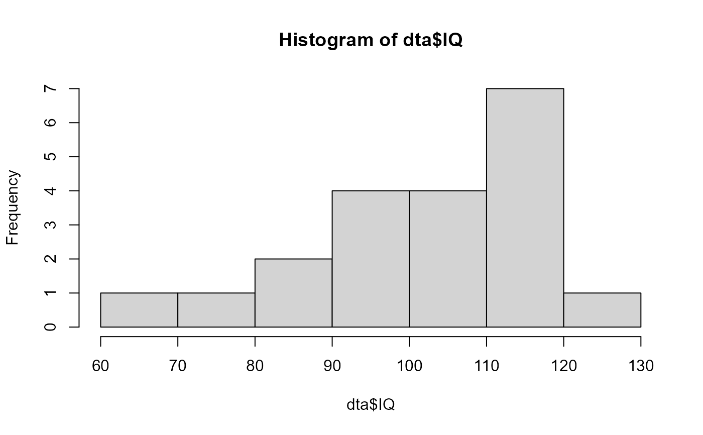
dta <- GRD(
RenameDV = "IQ",
SubjectsPerGroup = 20,
Population=list(
mean=100, # will set GM to 100
stddev=15 # will set STDDEV to 15
)
)
hist(dta$IQ)
# Examples for a between-subject design and for a within-subject design:
dta <- GRD( BSFactors = '3', SubjectsPerGroup = 20)
dta <- GRD( WSFactors = "Moment (2)", SubjectsPerGroup = 20)
# A complex, 3 x 2 x (2) mixed design with a variable amount of participants in the 6 groups:
dta <- GRD(BSFactors = "difficulty(3) : gender (2)",
WSFactors="day(2)",
SubjectsPerGroup=c(20,24,12,13,28,29)
)
# Defining population characteristics :
dta <- GRD(
RenameDV = "IQ",
SubjectsPerGroup = 20,
Population=list(
mean=100, # will set GM to 100
stddev=15 # will set STDDEV to 15
)
)
hist(dta$IQ)
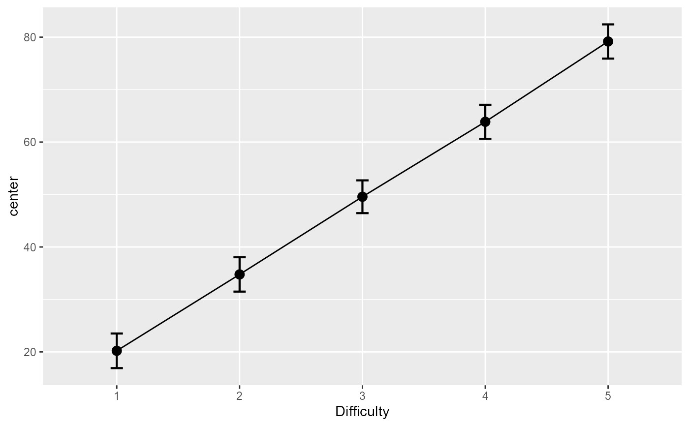
 # This example adds an effect along the "Difficulty" factor with a slope of 15
dta <- GRD(BSFactors="Difficulty(5)", SubjectsPerGroup = 100,
Population=list(mean=50,stddev=15),
Effects = list("Difficulty" = slope(15) ) )
# show the mean performance as a function of difficulty:
superb(DV ~ Difficulty, dta )
# This example adds an effect along the "Difficulty" factor with a slope of 15
dta <- GRD(BSFactors="Difficulty(5)", SubjectsPerGroup = 100,
Population=list(mean=50,stddev=15),
Effects = list("Difficulty" = slope(15) ) )
# show the mean performance as a function of difficulty:
superb(DV ~ Difficulty, dta )
 # An example in which the moments are correlated
dta <- GRD( BSFactors = "Difficulty(2)",WSFactors = "Moment (2)",
SubjectsPerGroup = 125,
Effects = list("Difficulty" = slope(3), "Moment" = slope(1) ),
Population=list(mean=50,stddev=20,rho=0.85)
)
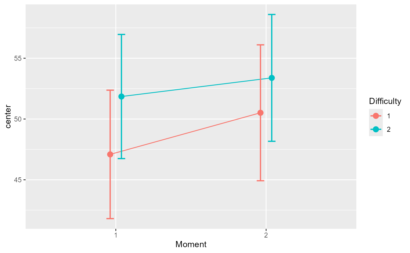
# the mean plot on the raw data...
superb(cbind(DV.1,DV.2) ~ Difficulty, dta, WSFactors = "Moment(2)",
plotLayout="line",
adjustments = list (purpose="difference") )
# An example in which the moments are correlated
dta <- GRD( BSFactors = "Difficulty(2)",WSFactors = "Moment (2)",
SubjectsPerGroup = 125,
Effects = list("Difficulty" = slope(3), "Moment" = slope(1) ),
Population=list(mean=50,stddev=20,rho=0.85)
)
# the mean plot on the raw data...
superb(cbind(DV.1,DV.2) ~ Difficulty, dta, WSFactors = "Moment(2)",
plotLayout="line",
adjustments = list (purpose="difference") )
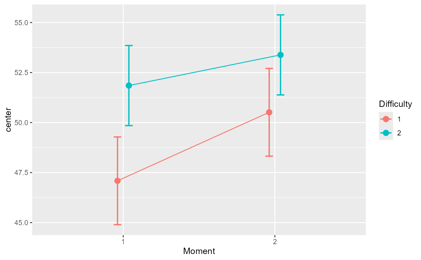
 # ... and the mean plot on the decorrelated data;
# because of high correlation, the error bars are markedly different
superb(cbind(DV.1,DV.2) ~ Difficulty, dta, WSFactors = "Moment(2)",
plotLayout="line",
adjustments = list (purpose="difference", decorrelation = "CM") )
# ... and the mean plot on the decorrelated data;
# because of high correlation, the error bars are markedly different
superb(cbind(DV.1,DV.2) ~ Difficulty, dta, WSFactors = "Moment(2)",
plotLayout="line",
adjustments = list (purpose="difference", decorrelation = "CM") )
 # This example creates a dataset in a 3 x 2 design. It has various effects,
# one effect of difficulty, with an overall effect of 10 more (+3.33 per level),
# one effect of gender, whose slope is 10 points (+10 points for each additional gender),
# and finally one interacting effect, which is 0 for the last three cells of the design:
GRD(
SubjectsPerGroup = 10,
BSFactors = c("difficulty(3)","gender(2)"),
Population = list(mean=100,stddev=15),
Effects = list(
"difficulty" = extent(10),
"gender"=slope(10),
"difficulty*gender"=custom(-300,+200,-100,0,0,0)
)
)
#> id difficulty gender DV
#> 1 1 1 1 -200.0223696
#> 2 2 1 1 -249.3466456
#> 3 3 1 1 -219.0164253
#> 4 4 1 1 -194.7836695
#> 5 5 1 1 -212.0825977
#> 6 6 1 1 -209.4928309
#> 7 7 1 1 -202.2625670
#> 8 8 1 1 -211.1262396
#> 9 9 1 1 -220.5218030
#> 10 10 1 1 -226.5086224
#> 11 11 2 1 261.5985389
#> 12 12 2 1 292.2302495
#> 13 13 2 1 302.5247186
#> 14 14 2 1 286.1920752
#> 15 15 2 1 303.3421736
#> 16 16 2 1 306.7561570
#> 17 17 2 1 301.0057046
#> 18 18 2 1 260.7710280
#> 19 19 2 1 291.8921049
#> 20 20 2 1 298.9531731
#> 21 21 3 1 1.6486957
#> 22 22 3 1 9.5645597
#> 23 23 3 1 -2.7668804
#> 24 24 3 1 9.1049384
#> 25 25 3 1 -11.4401333
#> 26 26 3 1 10.0258975
#> 27 27 3 1 -0.4283003
#> 28 28 3 1 -3.1923952
#> 29 29 3 1 38.4763633
#> 30 30 3 1 -9.9481251
#> 31 31 1 2 134.2274265
#> 32 32 1 2 107.5361201
#> 33 33 1 2 102.9429423
#> 34 34 1 2 107.5550510
#> 35 35 1 2 78.7100419
#> 36 36 1 2 127.8409616
#> 37 37 1 2 133.0170202
#> 38 38 1 2 98.1560319
#> 39 39 1 2 85.7758471
#> 40 40 1 2 82.9873138
#> 41 41 2 2 94.9377015
#> 42 42 2 2 94.8289361
#> 43 43 2 2 109.9420178
#> 44 44 2 2 98.7263524
#> 45 45 2 2 49.9305010
#> 46 46 2 2 89.5540670
#> 47 47 2 2 98.6437490
#> 48 48 2 2 118.8577957
#> 49 49 2 2 94.6632505
#> 50 50 2 2 88.1469122
#> 51 51 3 2 129.3325018
#> 52 52 3 2 124.4924055
#> 53 53 3 2 88.7067766
#> 54 54 3 2 112.2720658
#> 55 55 3 2 80.4664652
#> 56 56 3 2 122.9787756
#> 57 57 3 2 79.6919419
#> 58 58 3 2 98.2143983
#> 59 59 3 2 121.2413107
#> 60 60 3 2 93.1783347
# This last example creates a single group dataset,
# The instrument is assumed to return readings to
# plus or minus 0.1 only
GRD(
SubjectsPerGroup = 10,
Population = list(mean=100,stddev=15),
Instrument = list(
precision = 0.1, range = c(+0,+200)
)
)
#> id DV
#> 1 1 108.7
#> 2 2 108.9
#> 3 3 94.7
#> 4 4 84.6
#> 5 5 109.2
#> 6 6 86.0
#> 7 7 99.9
#> 8 8 103.3
#> 9 9 102.9
#> 10 10 102.6
# This example creates a dataset in a 3 x 2 design. It has various effects,
# one effect of difficulty, with an overall effect of 10 more (+3.33 per level),
# one effect of gender, whose slope is 10 points (+10 points for each additional gender),
# and finally one interacting effect, which is 0 for the last three cells of the design:
GRD(
SubjectsPerGroup = 10,
BSFactors = c("difficulty(3)","gender(2)"),
Population = list(mean=100,stddev=15),
Effects = list(
"difficulty" = extent(10),
"gender"=slope(10),
"difficulty*gender"=custom(-300,+200,-100,0,0,0)
)
)
#> id difficulty gender DV
#> 1 1 1 1 -200.0223696
#> 2 2 1 1 -249.3466456
#> 3 3 1 1 -219.0164253
#> 4 4 1 1 -194.7836695
#> 5 5 1 1 -212.0825977
#> 6 6 1 1 -209.4928309
#> 7 7 1 1 -202.2625670
#> 8 8 1 1 -211.1262396
#> 9 9 1 1 -220.5218030
#> 10 10 1 1 -226.5086224
#> 11 11 2 1 261.5985389
#> 12 12 2 1 292.2302495
#> 13 13 2 1 302.5247186
#> 14 14 2 1 286.1920752
#> 15 15 2 1 303.3421736
#> 16 16 2 1 306.7561570
#> 17 17 2 1 301.0057046
#> 18 18 2 1 260.7710280
#> 19 19 2 1 291.8921049
#> 20 20 2 1 298.9531731
#> 21 21 3 1 1.6486957
#> 22 22 3 1 9.5645597
#> 23 23 3 1 -2.7668804
#> 24 24 3 1 9.1049384
#> 25 25 3 1 -11.4401333
#> 26 26 3 1 10.0258975
#> 27 27 3 1 -0.4283003
#> 28 28 3 1 -3.1923952
#> 29 29 3 1 38.4763633
#> 30 30 3 1 -9.9481251
#> 31 31 1 2 134.2274265
#> 32 32 1 2 107.5361201
#> 33 33 1 2 102.9429423
#> 34 34 1 2 107.5550510
#> 35 35 1 2 78.7100419
#> 36 36 1 2 127.8409616
#> 37 37 1 2 133.0170202
#> 38 38 1 2 98.1560319
#> 39 39 1 2 85.7758471
#> 40 40 1 2 82.9873138
#> 41 41 2 2 94.9377015
#> 42 42 2 2 94.8289361
#> 43 43 2 2 109.9420178
#> 44 44 2 2 98.7263524
#> 45 45 2 2 49.9305010
#> 46 46 2 2 89.5540670
#> 47 47 2 2 98.6437490
#> 48 48 2 2 118.8577957
#> 49 49 2 2 94.6632505
#> 50 50 2 2 88.1469122
#> 51 51 3 2 129.3325018
#> 52 52 3 2 124.4924055
#> 53 53 3 2 88.7067766
#> 54 54 3 2 112.2720658
#> 55 55 3 2 80.4664652
#> 56 56 3 2 122.9787756
#> 57 57 3 2 79.6919419
#> 58 58 3 2 98.2143983
#> 59 59 3 2 121.2413107
#> 60 60 3 2 93.1783347
# This last example creates a single group dataset,
# The instrument is assumed to return readings to
# plus or minus 0.1 only
GRD(
SubjectsPerGroup = 10,
Population = list(mean=100,stddev=15),
Instrument = list(
precision = 0.1, range = c(+0,+200)
)
)
#> id DV
#> 1 1 108.7
#> 2 2 108.9
#> 3 3 94.7
#> 4 4 84.6
#> 5 5 109.2
#> 6 6 86.0
#> 7 7 99.9
#> 8 8 103.3
#> 9 9 102.9
#> 10 10 102.6