(advanced) Alternate ways to decorrelate repeated measures from transformations
Source:vignettes/Vignette8.Rmd
Vignette8.RmdThe methods CM (Cousineau, 2005;
Morey, 2008) and LM (Loftus
& Masson, 1994) can be unified when the transformations they
required are considered. In the Cousineau-Morey method, the raw data
must be subject-centered and bias-corrected.
Subject centering is obtained from
in which and where is the number of participants and is the number of repeated measures (sometimes noted with ).
Bias-correction is obtained from
These two operations can be performed with two matrix
transformations. In comparison, the LM method requires one
additional step, that is, pooling standard deviation, also achievable
with the following transformation.
in which is the variance in measurement and is the pooled variance across all mesurements.
With this approach, we can categorize all the proposals to repeated measure precision as requiring or not certain transformations. Table 1 shows these.
Table 1. Transformations required to implement one of the repeated-measures method. Preprocessing must precede post-processing
| Method | preprocessing | postprocessing | |
|---|---|---|---|
| Stand-alone | - | - | |
| Cousineau, 2005 | Subject-centering | - | - |
| CM | Subject-centering | Bias-correction | |
| NKM | Subject-centering | - | pool standard deviations |
| LM | Subject-centering | Bias-correction | pool standard deviations |
From that point of view, we see that the Nathoo, Kilshaw and Masson NKM (Nathoo, Kilshaw, & Masson, 2018; but see Heck, 2019) method is missing a bias-correction transformation, which explains why these error bars are shorter. The original proposal found in Cousineau, 2005, is also missing the bias correction step, which led Morey (2008) to supplement this approach. With these four approaches, we have exhausted all the possible combinations regarding decorrelation methods based on subject-centering.
We added two arguments in superbPlot to handle this transformation
approach, the first is preprocessfct and the second is
postprocessfct.
Assuming a dataset dta with replicated measures stored in say columns
called Score.1, Score.2 and
Score.3, the command
pCM <- superb(
    crange(Score.1,Score.3) ~ .,
    dta, WSFactors = "moment(3)",
    adjustments=list(decorrelation="none"),
    preprocessfct = "subjectCenteringTransform",
    postprocessfct = "biasCorrectionTransform",
    plotLayout = "pointjitter",
    errorbarParams = list(color="red", width= 0.1, position = position_nudge(-0.05) )
)
will reproduce the CM error bars because it decorrelates
the data as per this method. With one additional transformation,
pLM <- superb(
    crange(Score.1,Score.3) ~ .,
    dta, WSFactors = "moment(3)",
    adjustments=list(decorrelation="none"),
    preprocessfct = "subjectCenteringTransform",
    postprocessfct = c("biasCorrectionTransform","poolSDTransform"),
    plotLayout = "line",
    errorbarParams = list(color="orange", width= 0.1, position = position_nudge(-0.0) )
)
the LM method is reproduced. Finally, if the
biasCorrectionTransform is omitted, we get the NKM error
bars with:
pNKM <- superb(
    crange(Score.1,Score.3) ~ .,
    dta, WSFactors = "moment(3)",
    adjustments=list(decorrelation="none"),
    preprocessfct = "subjectCenteringTransform",
    postprocessfct = c("poolSDTransform"),
    plotLayout = "line",
    errorbarParams = list(color="blue", width= 0.1, position = position_nudge(+0.05) )
)
In what follow, I justapose the three plots to see the differences:
tlbl <- paste( "(red)    Subject centering & Bias correction == CM\n",
               "(orange) Subject centering, Bias correction & Pooling SDs == LM\n",
               "(blue)   Subject centering & Pooling SDs == NKM", sep="")

ornate <- list(
    xlab("Group"),
    ylab("Score"),
    labs(   title=tlbl),
    coord_cartesian( ylim = c(12,18) ),
    theme_light(base_size=10)
)

# the plots on top are made transparent
pCM2 <- ggplotGrob(pCM + ornate)
pLM2 <- ggplotGrob(pLM + ornate + makeTransparent() )
pNKM2 <- ggplotGrob(pNKM + ornate + makeTransparent() )

# put the grobs onto an empty ggplot
ggplot() +
    annotation_custom(grob=pCM2) +
    annotation_custom(grob=pLM2) +
    annotation_custom(grob=pNKM2)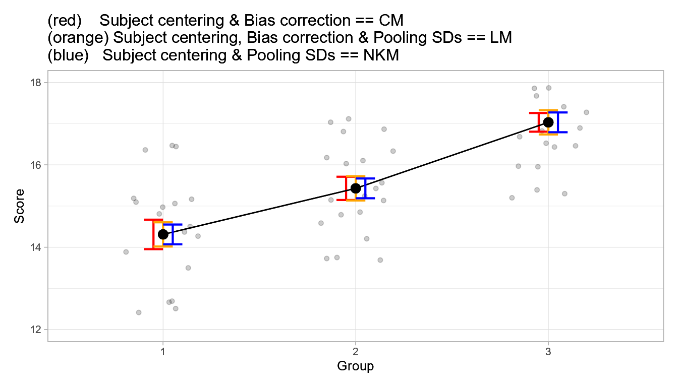
Figure 1. Plot of the tree decorrelation methods based on subject transformation.
The method from Cousineau (2005) missing the bias-correction step is not shown as it should not be used.
In summary
All the decorrelation methods based on transformations have (probably) been explored. An alternative approach using correlation was proposed in Cousineau (2019). All these approaches requires sphericity of the data. Other approaches are required to overcome this sphericity limitations.