In this vignette, we show how the Cohen’s can be illustrated. See Goulet-Pelletier & Cousineau (2018); Cousineau & Goulet-Pelletier (2020) for comprehensive reviews.
What is the Cohen’s ?
The Cohen’s , also known as the standardized mean difference (smd), is a standardized measure of effect size for pairwise conditions. It is standardized using the standard deviation, so that it ressemble a z scores. Often, the sign of the Cohen’s is removed, but it could be positive or negative; it is not bounded but usually, it is smaller than 1.
As an example, a Cohen’s of 0.5 indicates that the two group’s means are separated by 0.5 standard deviations. If you illustrate the two populations with normal, bell-shape, curves, then their mode would be visibly separated, indicating a sizeable difference between the two populations. Cohen would call this a medium effect (although in my opinion, this is already a large effect; any non-trivially small samples would find this difference significant). With a Cohen’s of 0.25, it is harder to see a difference between the two populations.
This descriptive statistic is computed from two groups (or two repeated measures) with
where is the pooled standard deviation across the two group’s standard deviations.
Illustrating this measure with a plot is difficult as it is a pairwise statistic. For example, if there is 5 groups, that represents 15 pairs of groups and consequently, 15 Cohen’s .
Here, we propose an alternative representation through an indirect statistic, using (Goulet-Pelletier & Cousineau, 2018). It is given by
where is the standard deviation in the group (here labeled “1”). The quantity is a baseline measure. It can be any value based on prior knowledge of the measure (for example, if the measures are IQ, then would be set to 100). Alternatively, it can also be the grand mean across all the conditions. This is the solution we adopt herein.
The statistic is a univariate measure, i.e., it is based on a single group’s data. Hence, in a plot, you could illustrate one per group.
Why is it interesting? The point is that the difference between two is the Cohen’s ! Likewise, the difference-adjusted confidence interval of is the same as the confidence interval of a Cohen’s . Hence, in a single plot, it is possible to derive all the Cohen’s and their significance.
Plotting with its confidence interval
Let’s define this statistic and its confidence interval estimator:
library(sadists) # for computing confidence intervals of Cohen's d
library(superb)

d1 <- function(X) {
        # the global variable GM.d1 is obtained from the initializer
        mean(X - GM.d1) / sd(X)
    }

CI.d1 <- function(X, gamma = .95) {
    n    <- length(X)
    dlow <- qlambdap(1/2-gamma/2, df = n-1, t = d1(X) * sqrt(n) )
    dhig <- qlambdap(1/2+gamma/2, df = n-1, t = d1(X) * sqrt(n) )
    c(dlow, dhig) / sqrt(n)
}
In that function, we have the variable GM.d1 which
represents the grand mean over all the condition. We see later how this
variable is initialized.
In what follow, I use a randomly-generated data with
GRD() simulating three dosage levels in a between-group
design. The three groups have different means of 50, 51.2 and 52.4 which
should translate into observed
of about 0.12 (between group 1 and group 2 as well as between group 2
and group 3) as the standard deviation in the population is 10:
# let's generate random data with true Cohen's dp
# of 0.12 (groups 1 and 2) and 0.24 (groups 1 and 3)
dta <- GRD( BSFactors = "Dose(3)",
    RenameDV          = "score",
    Effects           = list("Dose" = custom(0, 1.2, 2.4)),
    SubjectsPerGroup  = 500,
    Population        = list( mean = 50, stddev = 10)
)
## ------------------------------------------------------------
## Design is: 3 with 3 independent groups.
## ------------------------------------------------------------
## 1.Between-Subject Factors ( 3 groups ) :
## Dose; levels: 1, 2, 3
## 2.Within-Subject Factors ( 1 repeated measures ):
## 3.Subjects per group ( 1500 total subjects ):
## 500
## ------------------------------------------------------------If we set manually GM.d1 to the grand mean, we are ready
to make a plot. Alternatively, we can create an
initializer that will be run by
superbPlot() automatically. Here it is:
# the exact formulas for Cohen's d1 and dp. Only d1 is used in the plot
init.d1 <- function(df) {
        GM.d1 <<- mean(df$DV) # will make d1 relative to the grand mean
}
It will be run from the rawData data frame (generated by
superbPlot(); check superbData() if you want
to access that data frame) in which the measures are collated in the
column DV.
Now let’s make the plot, feeding d1 as the statistic
function:
# show a plot with Cohen's d1 and difference-adjusted confidence intervals of d1
superb(
    score ~ Dose,
    dta,
    statistic   = "d1",  errorbar  = "CI",
    gamma       = 0.95,
    plotLayout  = "line",
    adjustments = list(purpose="difference")
) + theme_light(base_size = 10) +
coord_cartesian( ylim = c(-0.3,+0.45) ) +
labs(title = "d_1 with difference-adjusted 95% confidence intervals of d_1",
     y     = "d_1 relative to grand mean")
## superb::FYI: Running initializer init.d1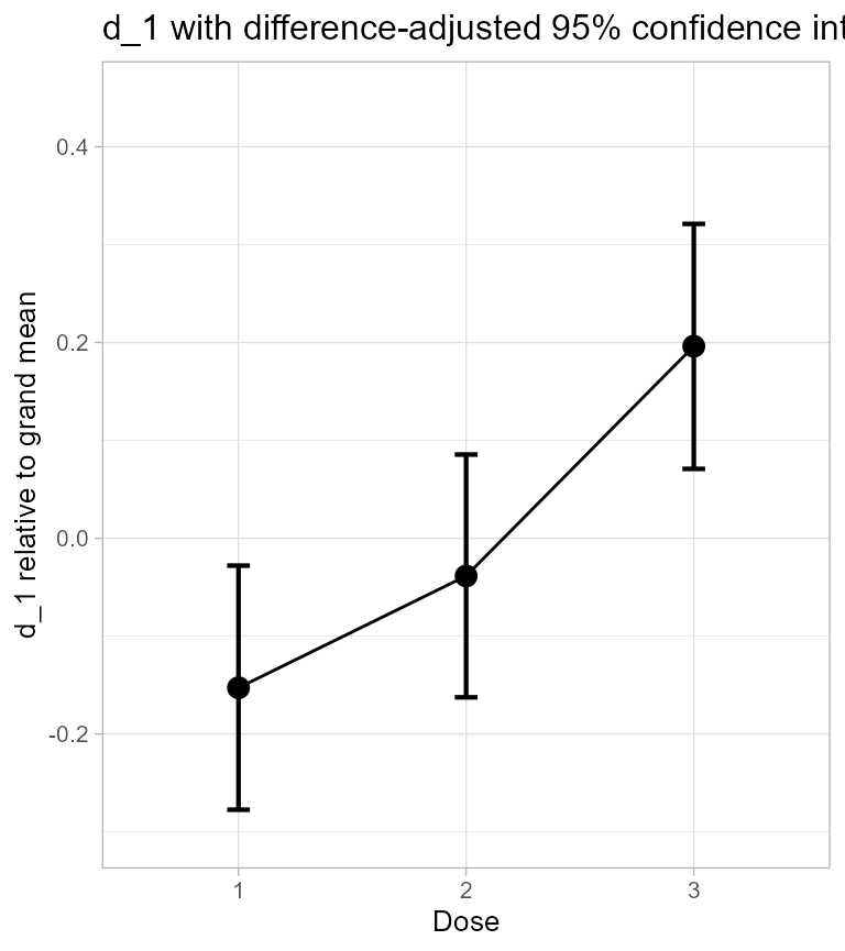
Figure 1. d_1 scores along with 95% confidence interval.
The difference between two is the Cohen’s and the difference-adjusted confidence intervals are adequate to compare two . For example, the of the first group is not included in the third group’s which indicates that the Cohen’s is significantly different from zero.
Note that in the above, the initializer was detected and run automatically. You can check that the initializer is detectable with
superb:::has.init.function("d1")## [1] TRUEChecking the results
To check the above, we could implement the formulas for the Cohen’s (Cousineau & Goulet-Pelletier, 2020):
dp <- function(X, Y) {
        mean(X - Y) / sqrt((length(X)*var(X) + length(Y)*var(Y))/(length(X)+length(Y)-2))
    }
CI.dp <- function(X, Y, gamma = .95) {
    n1 = length(X)
    n2 = length(Y)
    n = hmean(c(n1, n2))
    dlow <- qlambdap(1/2-gamma/2, df = n1+n2-2, t = dp(X, Y) * sqrt(n/2) )
    dhig <- qlambdap(1/2+gamma/2, df = n1+n2-2, t = dp(X, Y) * sqrt(n/2) )
    c(dlow, dhig) / sqrt(n/2)
}
Let’s extract the group’s data for intermediate computations:
grp1 <- dta$score[dta$Dose==1]
grp2 <- dta$score[dta$Dose==2]
grp3 <- dta$score[dta$Dose==3]
so that we can easily compute all three pairwise statistics:
dp12 <- round(dp(grp2, grp1), 3)
dp13 <- round(dp(grp3, grp1), 3)
dp23 <- round(dp(grp3, grp2), 3)
c(dp12, dp13, dp23)
## [1] 0.062 0.146 0.087… and their 95% confidence intervals:
cidp12 = round(CI.dp(grp2, grp1, 0.95), 3)
cidp13 = round(CI.dp(grp3, grp1, 0.95 ), 3)
cidp23 = round(CI.dp(grp3, grp2, 0.95 ), 3)
c(cidp12,cidp13,cidp23)
## [1] -0.062 0.186 0.022 0.270 -0.037 0.211Let’s put these numbers on the plot for easier examination using the
graphic directives showSignificance():
superb(
    score ~ Dose,
    dta,
    statistic  = "d1",  errorbar  = "CI", gamma     = 0.95,
    plotLayout = "line",
    adjustments = list(purpose="difference")
) + theme_light(base_size = 10) +
coord_cartesian( ylim = c(-0.3,+0.45) ) +
labs(title   = "d_1 with difference-adjusted 95% confidence intervals of d_1",
     caption = paste("Note: Cohen's d_p and its confidence interval computed with the \n",
                     "true formula (Cousineau & Goulet-Pelletier, 2020)"),
     y       = "d_1 relative to grand mean") +
showSignificance(c(1,2), 0.3, -0.01,
    paste("dp = ",dp12, ifelse(sign(cidp12[1])==sign(cidp12[2]),", p < .05",", p > .05")) ) +
showSignificance(c(1,3), 0.4, -0.01,
    paste("dp = ",dp13, ifelse(sign(cidp13[1])==sign(cidp13[2]),", p < .05",", p > .05"))) +
showSignificance(c(2,3), -0.25, +0.01,
paste("dp = ",dp23, ifelse(sign(cidp23[1])==sign(cidp23[2]),", p < .05",", p > .05"))) 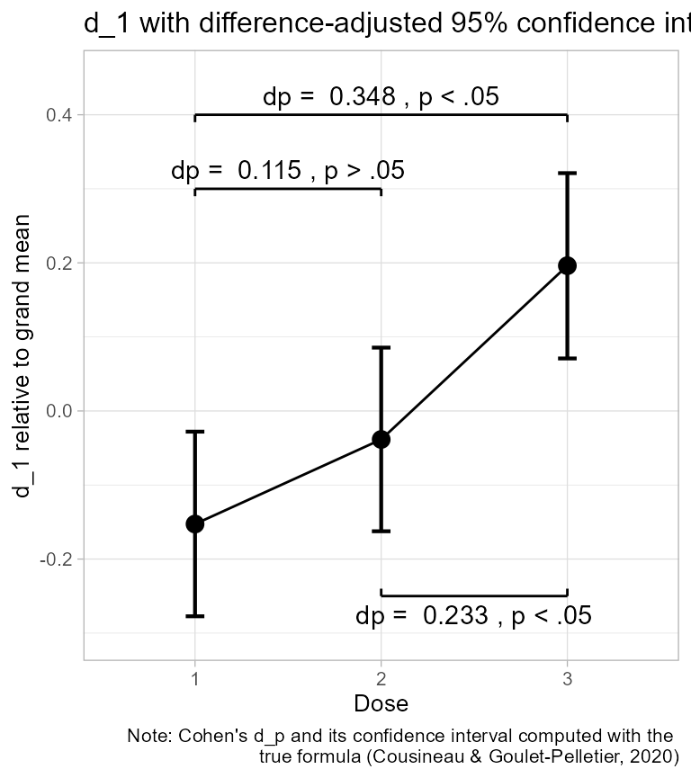
Figure 2. d_1 scores along with 95% confidence interval.
In the above, we used the fact that if both limits of the confidence interval are of the same sign, then they are on the same side with respect to zero, and therefore, excludes zero at a significance level of at least 5% (for 95% confidence intervals).
Let’s examine how good the difference-adjusted CI of are compared to the CI of . The following function (a) get the length of the Cohen’s interval; (b) average (in the square sense, see here) the two difference-adjusted confidence intervals of :
compareCIlength <- function(g1, g2) {
    # compute the Cohen's dp confidence interval length
    cilength.dp = round(CI.dp(g1, g2)[2]-CI.dp(g1, g2)[1], 3)

    # compute two d1 CI length, difference-adjusted
    len1    = sqrt(2)*(CI.d1(grp1)[2] - CI.d1(grp1)[1])
    len2    = sqrt(2)*(CI.d1(grp2)[2] - CI.d1(grp2)[1])
    # average in the square sense the two d1 CI lengths
    cilength.d1 = round(sqrt((len1^2 + len2^2)/2), 3)

    data.frame( dp.length = cilength.dp, d1.average.length = cilength.d1)
}

compareCIlength(grp1,grp2)
## dp.length d1.average.length
## 1 0.248 0.248
compareCIlength(grp1,grp3)## dp.length d1.average.length
## 1 0.248 0.248
compareCIlength(grp2,grp3)## dp.length d1.average.length
## 1 0.248 0.248As seen, there is no difference until the third decimal. The small difference comes from the fact that the degrees of freedom are separated, not pooled.