Data of Tulving, Mandler, & Baumal, 1964 (reproduction of 2021)

The data comes from Bradley-Garcia and 37 others (2021) . It is a near exact replication of the original study from (Tulving et al. 1964) .

The design is a (7) x 4 with: 7 levels of stimulus duration (within-subject) and 4 between-subject conditions. Additional variables included in the reproduction is the primary language of the participant in which he/she participated (mainly francophones and anglophones; and the gender (mainly male and female).

data(TMB1964r)

Format

An object of class data.frame.

References

Bradley-Garcia M, 37 others (2021). “The influence of exposure duration and context length on word recall: A replication of Tulving et al. (1964).” The Quantitative Methods for Psychology, 17(2), r1-r9. doi:10.20982/tqmp.17.2.r001 .

Tulving E, Mandler G, Baumal R (1964). “Interaction of two sources of information in tachistoscopic word recognition.” Canadian Journal of Psychology/Revue canadienne de psychologie, 18(1), 62.

Examples

library(ggplot2)

data(TMB1964r)

options(superb.feedback = 'none') # shut down 'warnings' and 'design' interpretation messages

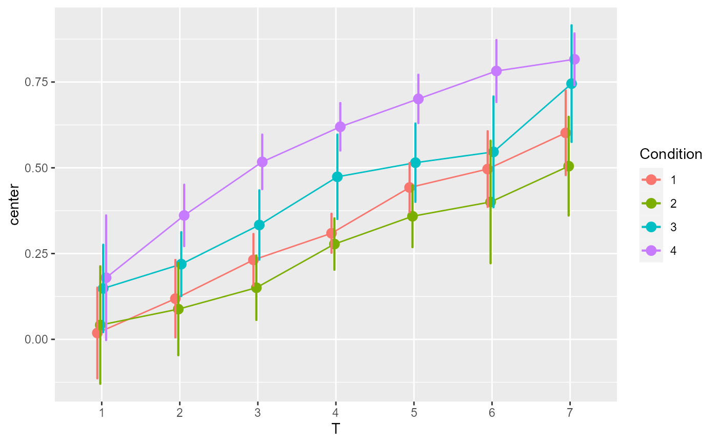
# general plot ignoring covariates sex and languages with only defaults
# We illustrate correlation- and difference-adjusted 95% confidence intervals of the mean
superb(
    crange(T1, T7) ~ Condition,
    TMB1964r,
    WSFactors = "T(7)",      # the within-subject factor (spanning 7 columns)
    adjustments = list(purpose="difference", decorrelation="CM"),
    plotLayout = "line"
)


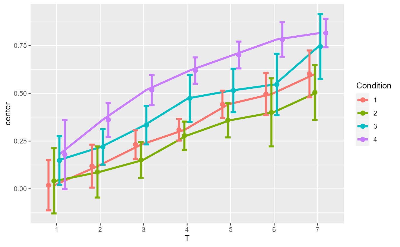
# We add directives for the error bars (thick), for the points (larger) and for the lines (thick)
plt <- superb(
    crange(T1, T7) ~ Condition,
    TMB1964r,
    WSFactors = "T(7)",
    adjustments = list(purpose="difference", decorrelation="CM"),
    plotLayout = "line", 
    errorbarParams = list(width = 0.5, linewidth=1.25, position = position_dodge(.5) ),
    pointParams = list(size=2.5, position = position_dodge(.5)),
    lineParams = list(linewidth=1.25)
)
plt


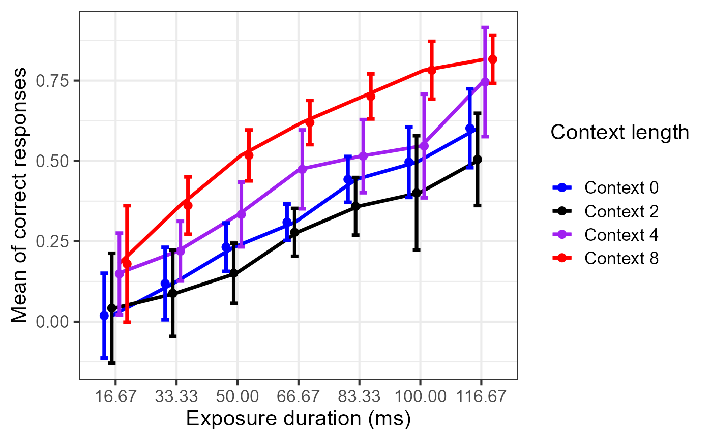
# Additional directives to set manually the colors, shapes, thick marks and labels.
plt + 
scale_colour_manual( 
    labels = c("Context 0", "Context 2", "Context 4", "Context 8"), 
    values = c("blue", "black", "purple", "red")) +
scale_shape_manual( 
    labels = c("Context 0", "Context 2", "Context 4", "Context 8"), 
    values = c("circle", "triangle", "square", "plus")) +
theme_bw(base_size = 16) +
labs(x = "Exposure duration (ms)", y = "Mean of correct responses", 
    colour = "Context length\n", shape = "Context length\n" ) + 
scale_x_discrete(labels=c("1" = "16.67", "2" = "33.33",
    "3"="50.00", "4" = "66.67", "5"="83.33", "6"="100.00", "7"="116.67"))




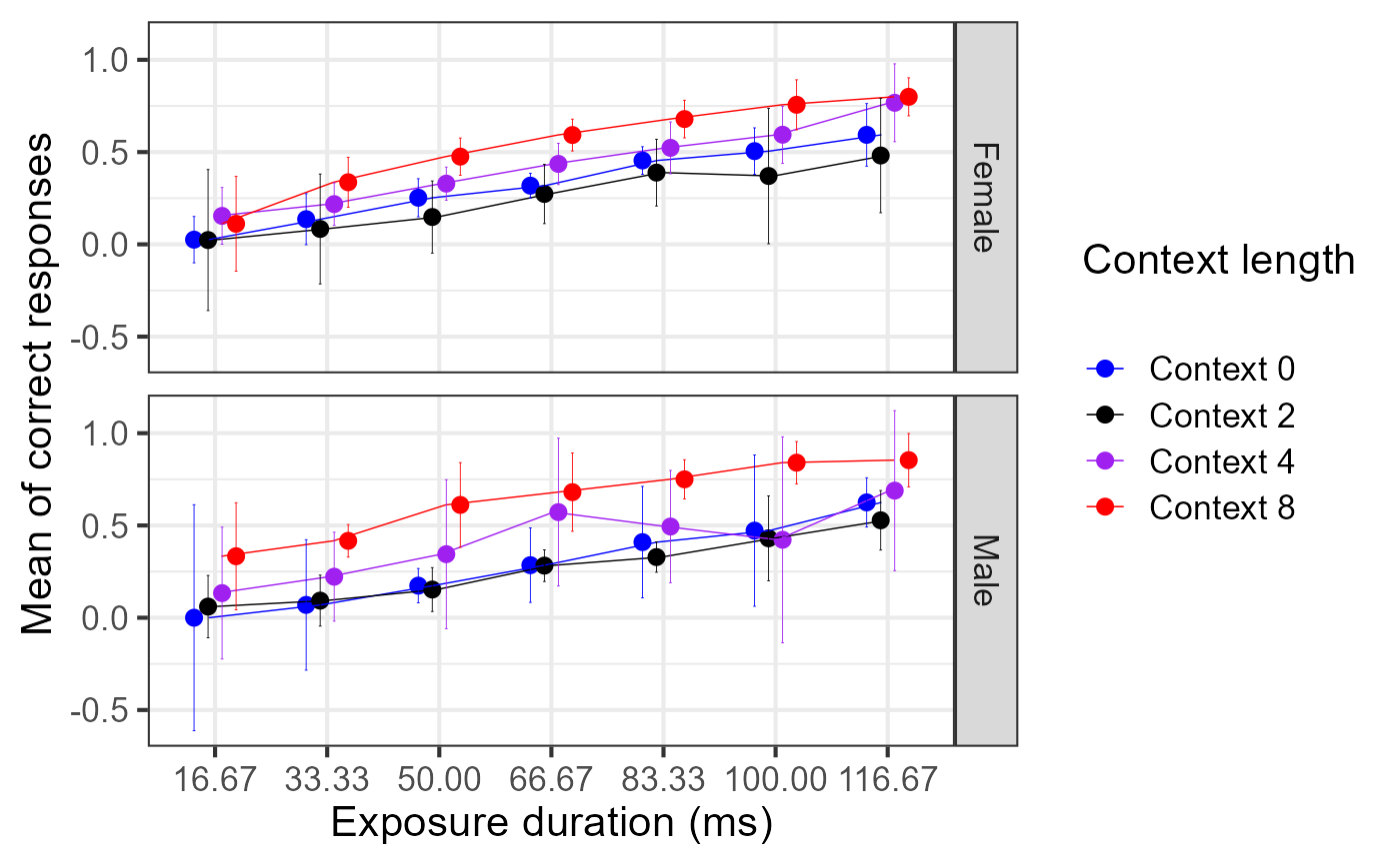
# Exploring three factors simultaneously: T, Condition and Sex (last two between-group)
superb(
    crange(T1, T7) ~ Condition + Sex,
    TMB1964r,
    WSFactors = "T(7)",      # the within-subject factor (spanning 7 columns)
    adjustments = list(purpose="difference", decorrelation="CM"),
    plotLayout = "line", 
    errorbarParams = list(linewidth=0.15, position = position_dodge(.5) ),
    pointParams = list(size=2.5, position = position_dodge(.5)),
    lineParams = list(linewidth=0.25)
) + 
scale_colour_manual( 
    labels = c("Context 0", "Context 2", "Context 4", "Context 8"), 
    values = c("blue", "black", "purple", "red")) +
scale_shape_manual( 
    labels = c("Context 0", "Context 2", "Context 4", "Context 8"), 
    values = c("circle", "triangle", "square", "plus")) +
theme_bw(base_size = 16) +
labs(x = "Exposure duration (ms)", y = "Mean of correct responses", 
    colour = "Context length\n", shape = "Context length\n" ) + 
scale_x_discrete(labels=c("1" = "16.67", "2" = "33.33",
    "3"="50.00", "4" = "66.67", "5"="83.33", "6"="100.00", "7"="116.67"))



#only keep 2 sex and 2 languages; the remaining cases are too sparse.
mee3 <- TMB1964r[(TMB1964r$Language != "I prefer not to answer")&TMB1964r$Language !="Other",]

### This last example is commented as CRAN servers are too slow
#
# advanced plots are available, such as pointjitter 
# and pointjitterviolin : a plot that superimposes the distribution as a violin plot
# 
# superb(
#   crange(T1, T7) ~ Condition + Language,
#   mee3,
#   WSFactors = "T(7)",
#   adjustments = list(purpose="difference", decorrelation="CM"), 
#   plotLayout = "pointjitterviolin",
#   jitterParams = list(alpha = 0.4), #near transparent jitter points
#   violinParams = list(alpha = 0.2)
#) + 
#scale_fill_manual( name = "Amount of context", 
#    labels = c("Context 0", "Context 2", "Context 4", "Context 8"), 
#    values = c("blue", "black", "purple", "red")) +
#scale_colour_manual( name = "Amount of context", 
#    labels = c("Context 0", "Context 2", "Context 4", "Context 8"), 
#    values = c("blue", "black", "purple", "red")) +
#scale_shape_manual( name = "Amount of context",
#    labels = c("Context 0", "Context 2", "Context 4", "Context 8"), 
#    values = c("circle", "triangle", "square", "cross")) +
#theme_bw(base_size = 16) +
#labs(x = "Exposure duration (ms)", y = "Mean of correct responses" )+ 
#scale_x_discrete(labels=c("1" = "16.67", "2" = "33.33",
#    "3"="50.00", "4" = "66.67", "5"="83.33", "6"="100.00", "7"="116.67"))
#