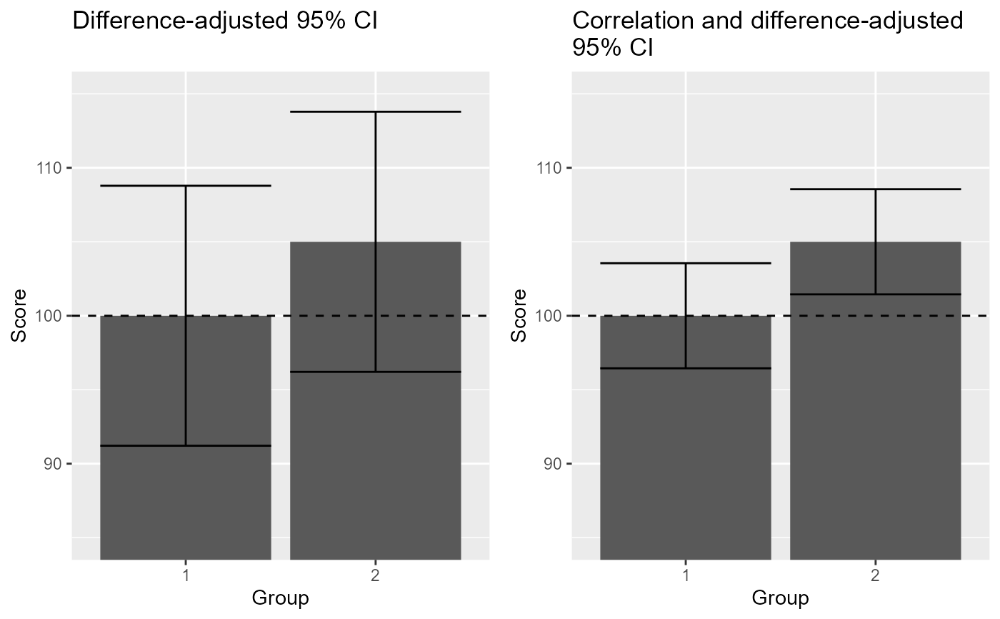
The data, taken from (Cousineau 2017) 7, is an example where the "stand-alone" 95\% confidence interval of the means returns a result in contradiction with the result of a statistical test. The paradoxical result is resolved by using adjusted confidence intervals, here the correlation- and different-adjusted confidence interval.
data(dataFigure2)Format
An object of class data.frame.
Source
References
Cousineau D (2017). “Varieties of confidence intervals.” Advances in Cognitive Psychology, 13, 140 – 155. doi:10.5709/acp-0214-z .
Examples
library(ggplot2)
library(gridExtra)
data(dataFigure2)

options(superb.feedback = 'none') # shut down 'warnings' and 'design' interpretation messages

## realize the plot with unadjusted (left) and ajusted (right) 95% confidence intervals
plt2a <- superb(
    cbind(pre, post) ~ .,
    dataFigure2,
    WSFactors = "Moment(2)",
    adjustments=list(purpose = "difference"),
    plotLayout="bar" ) +
  xlab("Group") + ylab("Score") + labs(title="Difference-adjusted 95% CI\n") +
  coord_cartesian( ylim = c(85,120) ) +
  geom_hline(yintercept = 100, colour = "black", linewidth = 0.5, linetype=2) +
  showSignificance( c(0.5, 2.5), 115, -1, "not significant???",
                    segmentParams = list( colour = "red" ) )
plt2b <- superb(
    cbind(pre, post) ~ .,
    dataFigure2,
    WSFactors = "Moment(2)",
    adjustments=list(purpose = "difference", decorrelation = "CA"),
    plotLayout="bar" ) +
  xlab("Group") + ylab("Score") + labs(title="Correlation and difference-adjusted\n95% CI") +
  coord_cartesian( ylim = c(85,120) ) +
  geom_hline(yintercept = 100, colour = "black", linewidth = 0.5, linetype=2)+
  showSignificance( c(0.5, 2.5), 115, -1, "highly significant!!!",
                    segmentParams = list( colour = "chartreuse3" ) )
plt2  <- grid.arrange(plt2a,plt2b,ncol=2)


## realise the correct t-test to see the discrepancy
t.test(dataFigure2$pre, dataFigure2$post, paired=TRUE)
#>
#> 	Paired t-test
#>
#> data:  dataFigure2$pre and dataFigure2$post
#> t = -2.9046, df = 24, p-value = 0.007776
#> alternative hypothesis: true mean difference is not equal to 0
#> 95 percent confidence interval:
#>  -8.552864 -1.447136
#> sample estimates:
#> mean difference
#>              -5
#>
## realise the correct t-test to see the discrepancy
t.test(dataFigure2$pre, dataFigure2$post, paired=TRUE)
#>
#> Paired t-test
#>
#> data: dataFigure2$pre and dataFigure2$post
#> t = -2.9046, df = 24, p-value = 0.007776
#> alternative hypothesis: true mean difference is not equal to 0
#> 95 percent confidence interval:
#> -8.552864 -1.447136
#> sample estimates:
#> mean difference
#> -5
#>