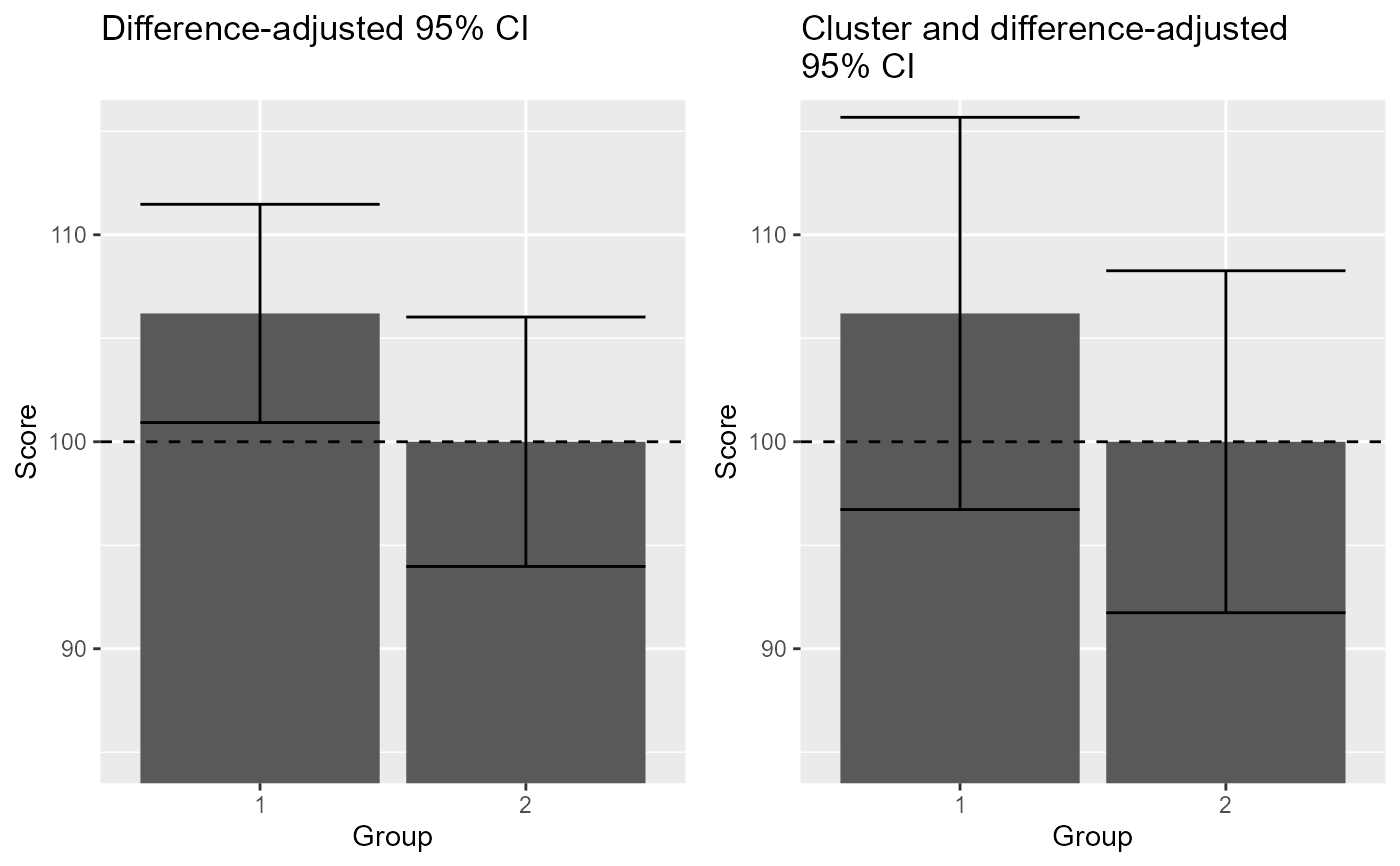
The data, inspired from (Cousineau and Laurencelle 2016) , is an example where the "stand-alone" 95\ a result in contradiction with the result of a statistical test. The paradoxical result is resolved by using adjusted confidence intervals, here the cluster- and different-adjusted confidence interval.
data(dataFigure3)Format
An object of class data.frame.
Source
References
Cousineau D, Laurencelle L (2016). “A Correction Factor for the Impact of Cluster Randomized Sampling and Its Applications.” Psychological Methods, 21, 121 – 135. doi:10.1037/met0000055 .
Examples
library(ggplot2)
library(gridExtra)
data(dataFigure3)

options(superb.feedback = 'none') # shut down 'warnings' and 'design' interpretation messages

## realize the plot with unadjusted (left) and ajusted (right) 95% confidence intervals
plt3a <- superb(
    VD ~ grp,
    dataFigure3,
    adjustments=list(purpose = "difference", samplingDesign = "SRS"),
    plotLayout="bar" ) +
  xlab("Group") + ylab("Score") + labs(title="Difference-adjusted 95% CI\n") +
  coord_cartesian( ylim = c(85,120) ) +
  geom_hline(yintercept = 100, colour = "black", linewidth = 0.5, linetype=2)+
  showSignificance( c(0.5, 2.5), 115, -1, "significant???",
                    segmentParams = list( colour = "red" ) )
plt3b <- superb(
    VD ~ grp,
    dataFigure3,
    adjustments=list(purpose = "difference", samplingDesign = "CRS"),
    plotLayout="bar", clusterColumn = "cluster" ) +
  xlab("Group") + ylab("Score") + labs(title="Cluster and difference-adjusted\n95% CI") +
  coord_cartesian( ylim = c(85,120) ) +
  geom_hline(yintercept = 100, colour = "black", linewidth = 0.5, linetype=2)+
  showSignificance( c(0.5, 2.5), 117, -1, "not significant!!!",
                    segmentParams = list( colour = "chartreuse3" ) )
plt3  <- grid.arrange(plt3a,plt3b,ncol=2)


## realise the correct t-test to see the discrepancy
res   <- t.test(dataFigure3$VD[dataFigure3$grp==1],
               dataFigure3$VD[dataFigure3$grp==2],
               var.equal=TRUE)
micc  <- mean(c(0.491334683772226, 0.20385744842838)) # mean ICC given by superbPlot
lam   <- CousineauLaurencelleLambda(c(micc, 5,5,5,5,5,5))
tcorr <- res$statistic / lam
pcorr <- 1-pt(tcorr,4)
# let's see the t value and its p value:
c(tcorr, pcorr)
#>         t         t
#> 1.4187225 0.1144879
## realise the correct t-test to see the discrepancy
res <- t.test(dataFigure3$VD[dataFigure3$grp==1],
dataFigure3$VD[dataFigure3$grp==2],
var.equal=TRUE)
micc <- mean(c(0.491334683772226, 0.20385744842838)) # mean ICC given by superbPlot
lam <- CousineauLaurencelleLambda(c(micc, 5,5,5,5,5,5))
tcorr <- res$statistic / lam
pcorr <- 1-pt(tcorr,4)
# let's see the t value and its p value:
c(tcorr, pcorr)
#> t t
#> 1.4187225 0.1144879