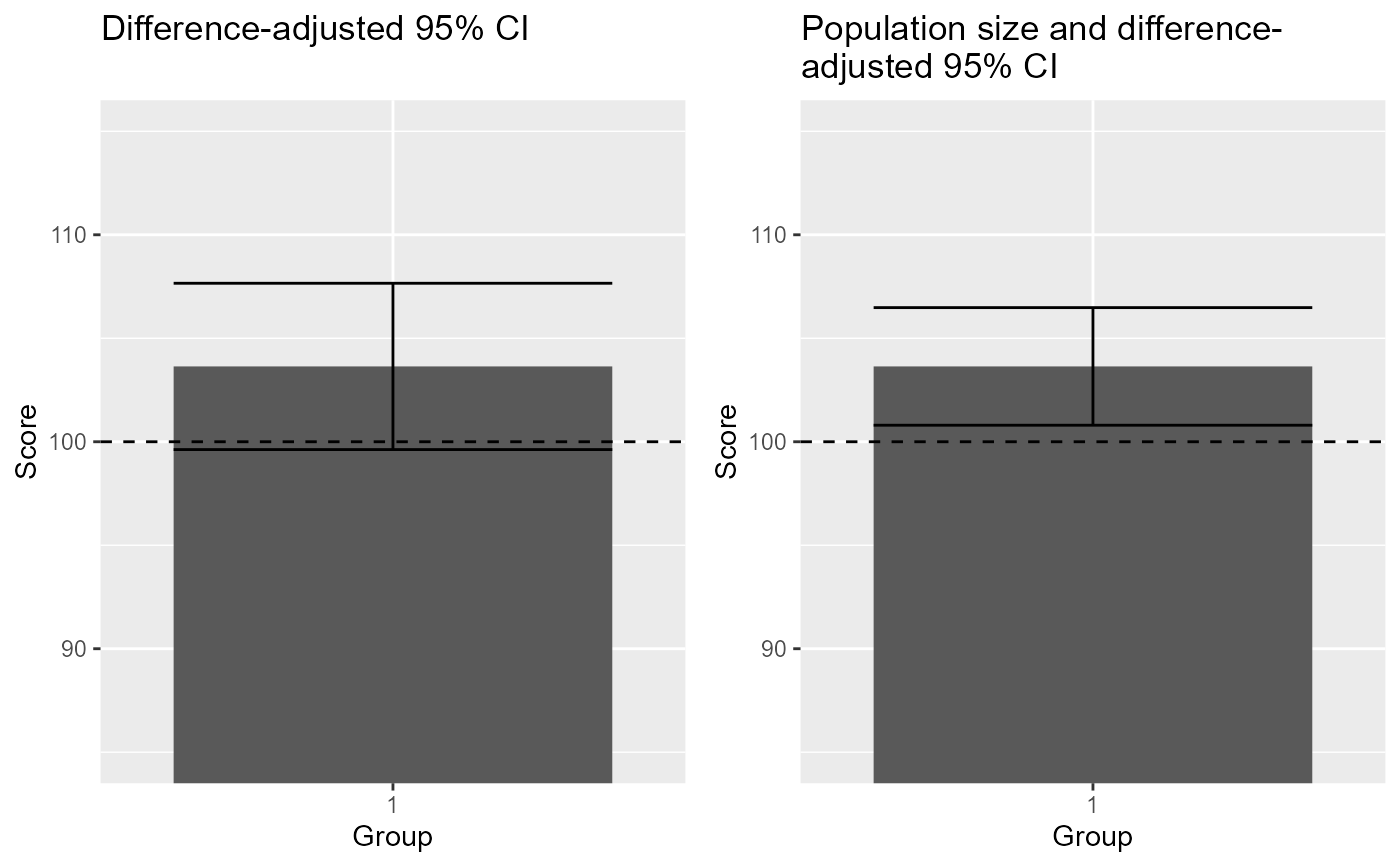
The data, inspired from Cousineau (2017) , shows an example where the "stand-alone" 95\ a result in contradiction with the result of a statistical test. The paradoxical result is resolved by using adjusted confidence intervals, here the population size-adjusted confidence interval.
data(dataFigure4)Format
An object of class data.frame.
Source
References
Cousineau D (2017). “Varieties of confidence intervals.” Advances in Cognitive Psychology, 13, 140 – 155. doi:10.5709/acp-0214-z .
Examples
library(ggplot2)
library(gridExtra)
data(dataFigure4)

options(superb.feedback = 'none') # shut down 'warnings' and 'design' interpretation messages

## realize the plot with unadjusted (left) and ajusted (right) 95% confidence intervals
plt4a = superb(
    score ~ group,
    dataFigure4,
    adjustments=list(purpose = "single", popSize = Inf),
    plotLayout="bar" ) +
  xlab("Group") + ylab("Score") + labs(title="Difference-adjusted 95% CI\n") +
  coord_cartesian( ylim = c(85,120) ) +
  geom_hline(yintercept = 100, colour = "black", linewidth = 0.5, linetype=2)+
  showSignificance( c(0.5, 1.5), 115, -1, "not significant???",
                    segmentParams = list( colour = "red" ) )
plt4b = superb(
    score ~ group,
    dataFigure4,
    adjustments=list(purpose = "single", popSize = 50 ),
    plotLayout="bar" ) +
  xlab("Group") + ylab("Score") + labs(title="Population size and difference-\nadjusted 95% CI") +
  coord_cartesian( ylim = c(85,120) ) +
  geom_hline(yintercept = 100, colour = "black", linewidth = 0.5, linetype=2)+
  showSignificance( c(0.5, 1.5), 115, -1, "highly significant!!!",
                    segmentParams = list( colour = "chartreuse3" ) )
plt4 = grid.arrange(plt4a,plt4b,ncol=2)


## realise the correct t-test to see the discrepancy
res = t.test(dataFigure4$score, mu=100)
tcorr = res$statistic /sqrt(1-25/50)
pcorr = 1-pt(tcorr,24)
c(tcorr, pcorr)
#>           t           t
#> 2.644354620 0.007100794
## realise the correct t-test to see the discrepancy
res = t.test(dataFigure4$score, mu=100)
tcorr = res$statistic /sqrt(1-25/50)
pcorr = 1-pt(tcorr,24)
c(tcorr, pcorr)
#> t t
#> 2.644354620 0.007100794