superbToWide: Reshape long data frame to wide, suitable for superbPlot
Source:R/superbToWide.R
superbToWide.RdThe function suberbToWide() is an extension to Navarro's WideToLong function
with ample checks to make sure all is legit, so that the data
is suitably organized for suberb. See Cousineau et al. (2021)
for more.
Other techniques are available to transform long to wide, but many asked for
this function to ship within superb. Note that with the function superb()
and a formula, there really is no need anymore to use superbToWide().
superbToWide(
  data,
  id = NULL,
  BSFactors = NULL,
  WSFactors = NULL,
  variable = NULL
)
Arguments
Value
A wide-format data frame ready for superbPlot() or superbData(). All other
variables will be erased.
References
Cousineau D, Goulet M, Harding B (2021). “Summary plots with adjusted error bars: The superb framework with an implementation in R.” Advances in Methods and Practices in Psychological Science, 4, 1–18. doi:10.1177/25152459211035109 .
Examples
library(ggplot2)
library(gridExtra)
# Example using the built-in dataframe Orange.
data(Orange)
superbToWide(Orange, id = "Tree", WSFactors = c("age"), variable = "circumference")
#> Tree circumference.118 circumference.484 circumference.664 circumference.1004
#> 1 3 30 51 75 108
#> 2 1 30 58 87 115
#> 3 5 30 49 81 125
#> 4 2 33 69 111 156
#> 5 4 32 62 112 167
#> circumference.1231 circumference.1372 circumference.1582
#> 1 115 139 140
#> 2 120 142 145
#> 3 142 174 177
#> 4 172 203 203
#> 5 179 209 214
# Optional: change column names to shorten "circumference" to "DV"
names(Orange) <- c("Tree","age","DV")
# turn the data into a wide format
Orange.wide <- superbToWide(Orange, id = "Tree", WSFactors = c("age"), variable = "DV")
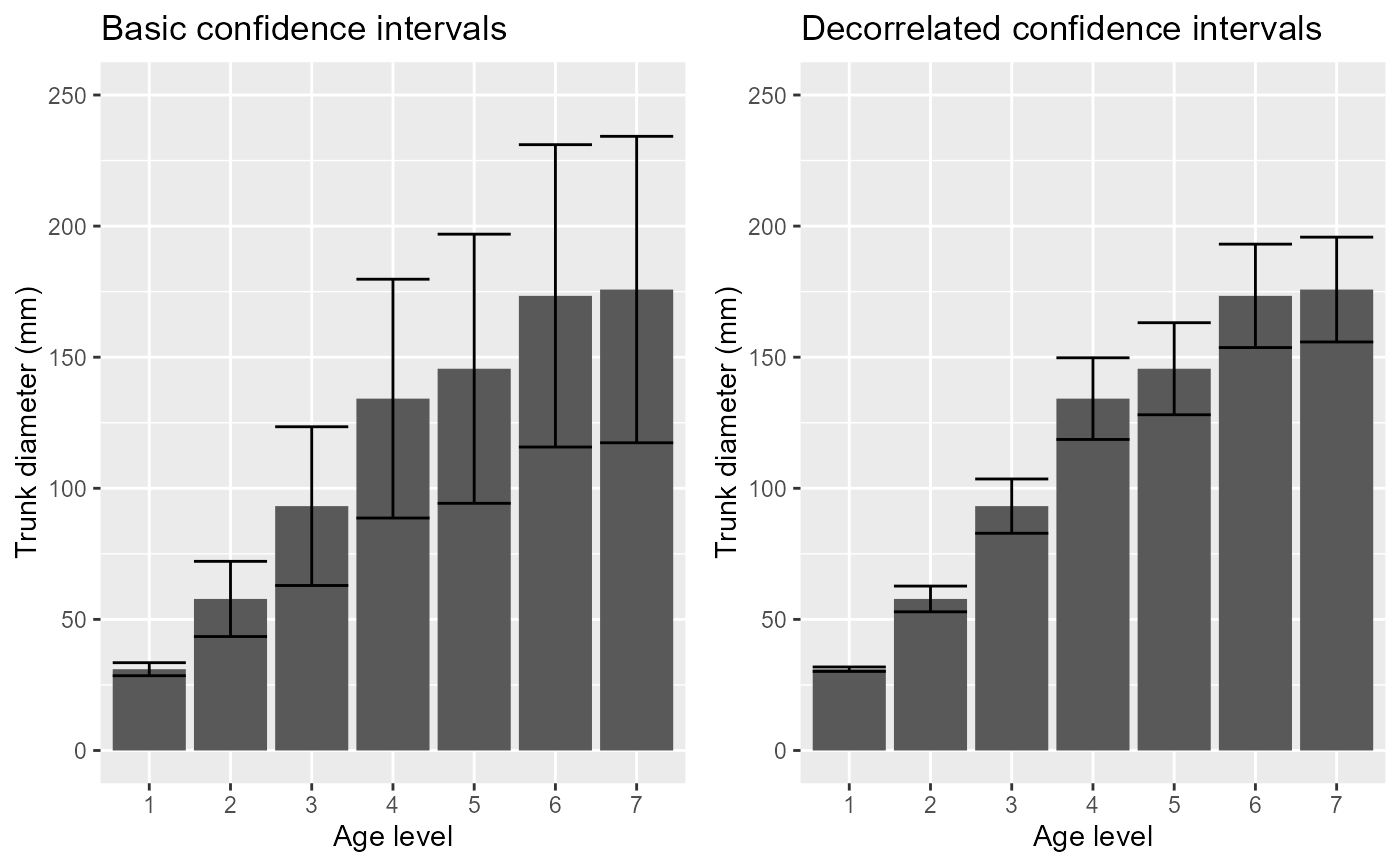
# Makes the plots two different way:
p1=superbPlot( Orange.wide, WSFactors = "age(7)",
variables = c("DV.118","DV.484","DV.664","DV.1004","DV.1231","DV.1372","DV.1582"),
adjustments = list(purpose = "difference", decorrelation = "none")
) +
xlab("Age level") + ylab("Trunk diameter (mm)") +
coord_cartesian( ylim = c(0,250) ) + labs(title="Basic confidence intervals")
p2=superbPlot( Orange.wide, WSFactors = "age(7)",
variables = c("DV.118","DV.484","DV.664","DV.1004","DV.1231","DV.1372","DV.1582"),
adjustments = list(purpose = "difference", decorrelation = "CA")
) +
xlab("Age level") + ylab("Trunk diameter (mm)") +
coord_cartesian( ylim = c(0,250) ) + labs(title="Decorrelated confidence intervals")
grid.arrange(p1,p2,ncol=2)
 # Note that with superb(), there is no need to reformat
# into a wide format anymore:
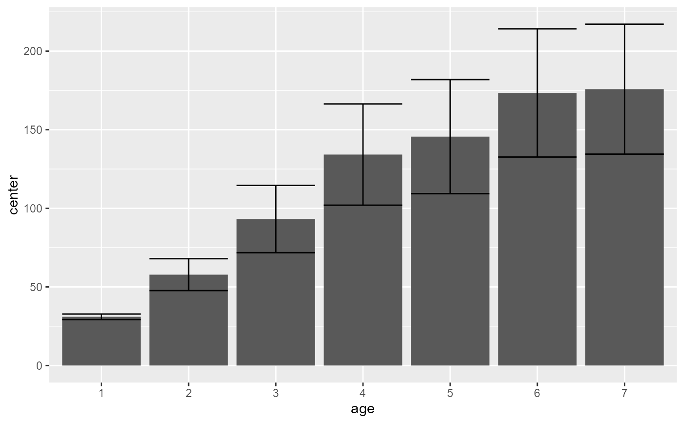
superb( DV ~ age | Tree, Orange )
# Note that with superb(), there is no need to reformat
# into a wide format anymore:
superb( DV ~ age | Tree, Orange )