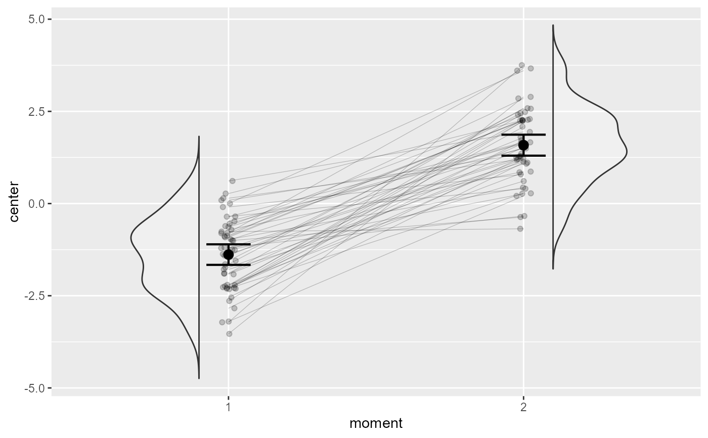
superbPlot comes with a few built-in templates for making the final plots. The corset plot is specifically devised for 2-repeated-measure design: it merges the "pointindividualline" layout with a raincloud layout (Belisario 2021) . All layout produces ggplot objects that can be further customized. Additionally, it is possible to create custom-make templates (see vignette 5). The functions, to be "superbPlot-compatible", must have these parameters:
Arguments
- summarydata
a data.frame with columns "center", "lowerwidth" and "upperwidth" for each level of the factors;
- xfactor
a string with the name of the column where the factor going on the horizontal axis is given;
- groupingfactor
a string with the name of the column for which the data will be grouped on the plot;
- addfactors
a string with up to two additional factors to make the rows and columns panels, in the form "fact1 ~ fact2";
- rawdata
always contains "DV" for each participants and each level of the factors;
- lineParams
(optional) list of graphic directives that are sent to the geom_line layer including the option colorize "bySlope", "byId" or "none";
- pointParams
(optional) list of graphic directives that are sent to the geom_bar layer;
- errorbarParams
(optional) list of graphic directives that are sent to the geom_superberrorbar layer;
- jitterParams
(optional) list of graphic directives that are sent to the geom_jitter layer;
- violinParams
(optional) list of graphic directives that are sent to the geom_boxplot layer;
- facetParams
(optional) list of graphic directives that are sent to the facet_grid layer;
- xAsFactor
(optional) Boolean to indicate if the factor on the horizontal should continuous or discrete (default is discrete).
Value
a ggplot object
References
Belisario K (2021). Corset Plots: Visualizing Heterogeneity in Change Outcomes Across Two Timepoints. doi:10.5281/zenodo.4905031 , https://cran.r-project.org/package=ggcorset.
Examples
# We first generate randomly a 2-measurement dataset with 50 participants and a large effect
dta <- GRD(SubjectsPerGroup = 50, WSFactors = "moment(2)", Effects = list("moment"=slope(3)))

# This will make a basic corset plot
superb(
   cbind(DV.1, DV.2) ~ .,
   dta,
   WSFactors = "moment(2)",
   plotLayout = "corset"
)


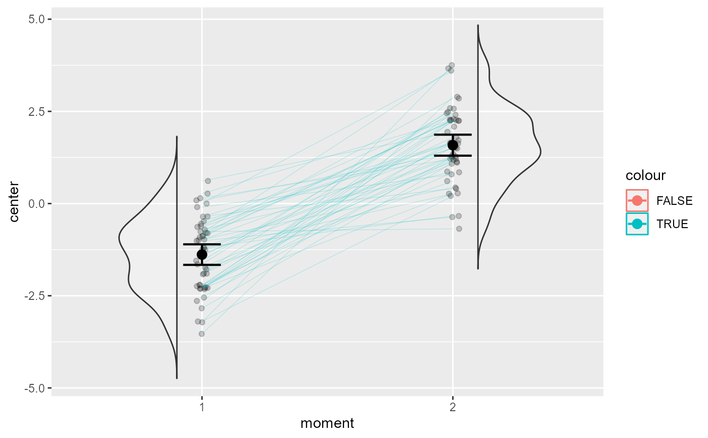
# This will color the increasing and decreasing individuals
superb(
   cbind(DV.1, DV.2) ~ .,
   dta,
   WSFactors = "moment(2)",
   plotLayout = "corset",
   lineParams = list(colorize="bySlope")
)


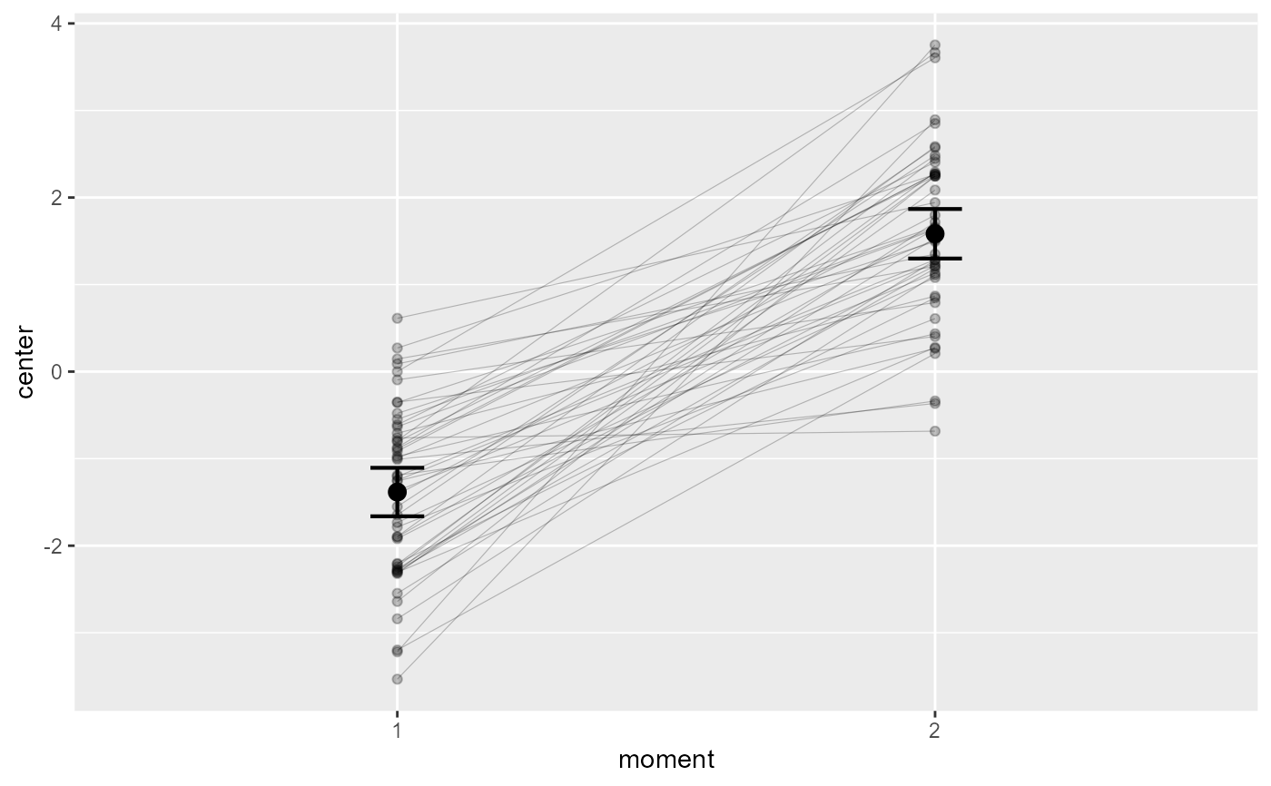
# This layout has similarities with the "pointindividualline" layout
superb(
   cbind(DV.1, DV.2) ~ .,
   dta,
   WSFactors = "moment(2)",
   plotLayout = "pointindividualline"
)


# if you extract the data with superbData, you can
# run this layout directly
processedData <- superb(
   cbind(DV.1, DV.2) ~ .,
   dta,
   WSFactors = "moment(2)",
   showPlot  = FALSE
)

superbPlot.corset(processedData$summaryStatistic,
   "moment", NULL, ".~.",
   processedData$rawData,
   lineParams = list(colorize="bySlope") )
