superbPlot 'lineBand' layout

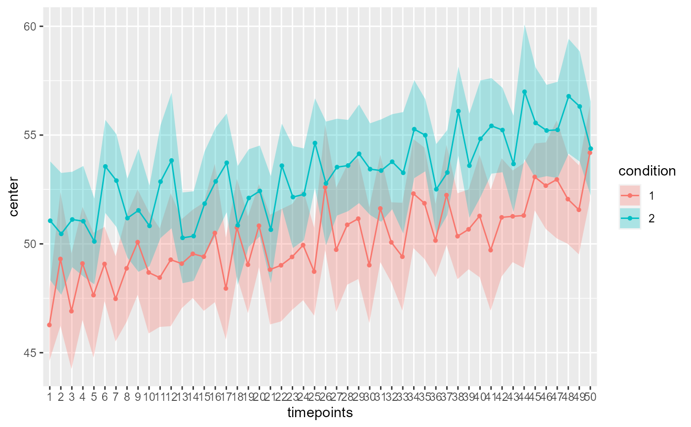
The lineBand layout displays an error band instead of individual error bars. This layout is convenient when you have many points on your horizontal axis (so that the error bars are difficult to distinguish) and when the results are fairly smooth.

The functions has these parameters:

superbPlot.lineBand(
  summarydata,
  xfactor,
  groupingfactor,
  addfactors,
  rawdata,
  pointParams = list(),
  lineParams = list(),
  facetParams = list(),
  errorbandParams = list(),
  xAsFactor = TRUE
)

Arguments

summarydata

a data.frame with columns "center", "lowerwidth" and "upperwidth" for each level of the factors;

xfactor

a string with the name of the column where the factor going on the horizontal axis is given;

groupingfactor

a string with the name of the column for which the data will be grouped on the plot;

addfactors

a string with up to two additional factors to make the rows and columns panels, in the form "fact1 ~ fact2";

rawdata

always contains "DV" for each participants and each level of the factors

pointParams

(optional) list of graphic directives that are sent to the geom_point layer

lineParams

(optional) list of graphic directives that are sent to the geom_jitter layer

facetParams

(optional) list of graphic directives that are sent to the facet_grid layer

errorbandParams

(optional) list of graphic directives that are sent to the geom_ribbon layer

xAsFactor

(optional) Boolean to indicate if the factor on the horizontal should continuous or discrete (default is discrete)

Value

a ggplot object

References

There are no references for Rd macro \insertAllCites on this help page.

Examples

# this creates a fictious time series at 100 time points obtained in two conditions:
dta <- GRD( WSFactors = "timepoints (50) : condition(2)", 
    SubjectsPerGroup = 20,
    RenameDV = "activation",
    Effects = list("timepoints" = extent(5), "condition" = extent(3) ),
    Population=list(mean=50,stddev=10,rho=0.75)
)

# This will make a plot with error band
superbPlot(dta, 
   WSFactors   = c("timepoints(50)", "condition(2)"),
   variables = colnames(dta)[2:101],   ## all the names of the dataframe except "id"
   adjustments = list(
        purpose       = "single",
        decorrelation = "CM"        ## or none for no decorrelation
   ),
   plotStyle="lineBand",            # note the uppercase B 
   pointParams = list(size= 1)      # making points smaller has better look
)


# if you extract the data with superbData, you can 
# run this layout directly
#processedData <- superbData(dta, 
#   WSFactors   = c("timepoints(100)", "condition(2)"), variables = colnames(dta)[2:201],
#   adjustments = list(
#        purpose       = "single",
#        decorrelation = "CM"        ## or none for no decorrelation
#   )
#)
#
#superbPlot.lineBand(processedData$summaryStatistic,
#   "timepoints",
#   "condition",
#   ".~.",
#   processedData$rawData)